Deep Learning Approach to Detect Banana Plant Diseases
Original Source Here
Deep Learning Approach to Detect Banana Plant Diseases
A system to identify Banana plant diseases at the early stages and to be aware of the diseases.
Introduction
Hello folks  This is my final year research project based on deep learning. Let me give an introduction about my project first.
When we talk about banana it’s a famous fruit that commonly available across the world, because it instantly boosts your energy. Bananas are one most consumed fruit in the world. According to modern calculations, Bananas are grown in around 107 countries since it makes a difference to lower blood pressure and to reduce the chance of cancer and asthma.
One of the problems that occur with banana cultivation is the number of diseases affecting the entire crop. To prevent such diseases most of the farmers use integrated chemicals and cultural methods.
Targeted Diseases to Identify
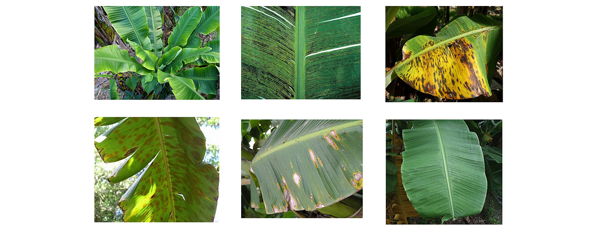
Banana plant diseases have become a severe problem in all over the world. The classical and ancient strategy for reconditioning and identifying banana plant diseases is based on bare eye observation.
The major diseases are “Cordana leafspot”, “Banana bunchy top”, “Banana streak”, “Banana sigatoka” and “Banana Speckle”.
So lets move on to coding to build a residual model
Develop a Residual Model to Identify Banana Plant Diseases
Here I will describe what a residual model is and the techniques I have used to augment the dataset. Tensorflow and Keras are the main libraries I have used.
The most important thing is to have a valid dataset for training and testing. I couldn’t find a proper dataset from Kaggle therefore I had to augment my dataset using openCV. The augmentation is as follows.
At the first step you need to import the necessary libraries first. This can be done either using conda or pip commands.
The next step is to initialize values for your model. For the training it’s a must have a clean dataset. At the first line of the code we need to setup following key features.
- Epoch Size = 35
- Learning_Rate = 0.001
- BS = 16
- Image_Dims = (224,224,3)
Make sure that you have a decent amount of images when setting up epoch size and batch size. Increasing the batch size will grab your memory power but give you better results.
Note: Recommended batch size is 16 or 32. If your memory power is low keep it as 10
The next step is to grab the image paths and to shuffle them randomly
Note: You can either use argument parser or the image path directly.
Then we need to load the input images and preprocess them and to save them in a data list.
The same thing with the labels, we need to extract the class labels from the image path and update them to a label list. As the next step we need to scale the raw pixel intensities to the range [0,1]
Here I’m using a LabelBinarizer() with the help of scikit-learn package to binarize the labels.
Note: You can either initialize you class labels manually as well.
Ex: Labels = [‘class1’, ‘class2, ‘class3’]
Here we didn’t use a separate dataset for devSet I have divided the dataset 80% for training and 20% for testing. Using the ImageDataGenerator I have done couple of augmentations as well.
The next part is to build your Residual model. For that I have created a separate python class. I will describe my ResidualNetwork class later. When there are more than two classes we have to choose “categorial_crossentropy” as the loss function and for the final dense layer we need to add ‘Softmax’ activation function as well.
Note: Final dense layer and the softmax function is in ResidualNetwork class:
Note: If you provide labels as integers make sure to choose “SparseCategoricalCrossentropy” loss, else it wont work properly.
I have used “SGD” Optimizer (Stochastic Gradient descent) as the loss function. To save the best weights of the model, keras has given Earlystoppings, Checkpoints and Best learning rate. ‘ReduceLROnPlateau’ is used to reduce learning rate when a metric has stopped improving.
After setting up everything you need to train the model. For that I’m using ‘model.fit_generator’.
Here I’m assigning value for ‘steps_per_epoch’ by dividing the trainX from the Batch_Size. Make sure to call your ‘call back list’ when training the network.
As the final step you need to save your model and the label binarizer to the disk. This can be done with the following code line.
model.save(args["model"], save_format="h5")f = open(args["labelbin"], "wb")
f.write(pickle.dumps(mlb))
f.close()
Now lets move to the Residual network model quickly. Soo Residual networks are combined with convolutional blocks. Haha… So don’t get confused………I will explain what’s a convolutional block is…
Residual Model Architecture
You have to pass your image input values to the 2Dconvolutional layer to produce tensor outputs. Starting with the filter size of ‘16’ with (3,3) kernal s is a good way and gradually you can increase that. This is the common block we need to implement. After this block we need three more convolutional blocks, and a skipping block.
Note: Make sure that you pass input values to the common block only
# Block 1
X = Conv2D(32, (3, 3), padding="same", strides=(1, 1), name="con_layer2")(X0)
X = BatchNormalization(axis=3, name="B2")(X)
X = Activation("relu")(X)
X = MaxPooling2D(pool_size=(1, 1), strides=(1, 1))(X)
So we need to to have three blocks like this to build the residual model. Skipping block is the next part after this. So make sure to add layers as well after implementing the skipping block.
Note: You need to add two more blocks(Block 1) like this..
So mainly a block consists with
- A main block
- Three convolutional blocks
- A skipping block
As the last step we need to add a flatten layer, dense layer and a dropout layer with 0.5 to avoid overfittings.
At last we need to return model to run the code……
You can evaluate your model by changing the number of layers, adjusting the learning rates, parameters as well. So I have plotted two graphs to evaluate my accuracy.
When deeply talking about the model which I used to train is consists with a Main common block , 9 Convolutional blocks and 3 skipping blocks. Simply I hope this drawing will relax your brain.
The final accuracy was around 98.8% which gave a smile to my face…
Increasing the number of layers wont give you good results it’ll try to overfit to your model. So I recommend you to use 6 blocks with 2 skipping blocks if you have less amount of images.
Unfortunately my GPU is not good so it took long time to train 
Have a nice Day!!
AI/ML
Trending AI/ML Article Identified & Digested via Granola by Ramsey Elbasheer; a Machine-Driven RSS Bot
via WordPress https://ramseyelbasheer.io/2021/07/31/deep-learning-approach-to-detect-banana-plant-diseases/