Data to Model to API: An End-to-End Approach
Original Source Here
Data to Model to API: An End-to-End Approach
Learn how to stitch the entire fabric of ML/DL life cycle stages together.
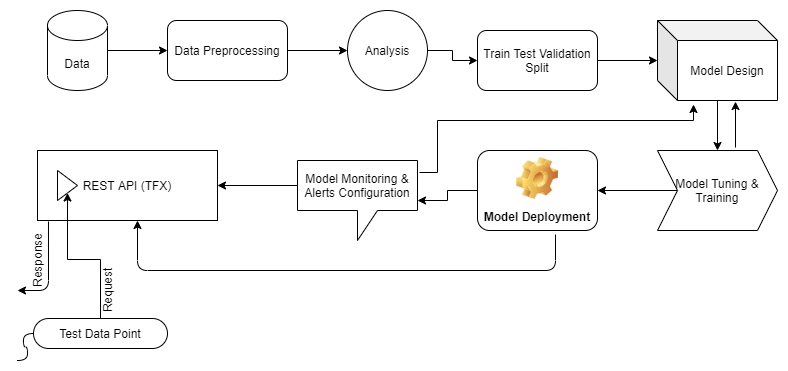
In this blog, we are not going to discuss the mighty Optimus Prime but we are going to go through the entire journey of a machine learning-based use case. We are going to start by data processing, move onto building a data pipeline to feed to model for training using Tensorflow, build a model architecture using a high-level tf.keras API and then finally serve the model using FastAPI. Also, we would use an alternative and more maintainable way of serving an ML model, TFX Serving an extended feature of Tensorflow APIs. This article does not talk about tuning ML models because the aim here is to learn the operationalization aspects of an ML model from start to finish.
The flow of the article is as follows:
- The Problem Statement
- Data Preprocessing
- Building a Data Pipeline
- Model Design, Training, and Evaluation
- Model Deployment (REST API) Using TFX Serving
The Problem Statement
We need to figure out a way to estimate the sentiment of a given tweet i.e. whether the tweet has a positive sentiment or a negative sentiment.
Now, the most basic way to solve this problem without using any ML techniques would be to make a frequency dictionary of words after removing insignificant stop words for both the classes (positive and negative) separately using the available annotated data. And, then for every tweet, after removing stop words as we did while building frequency dictionary, map the words in the tweet with their respective frequencies in both the classes, At the end, we could just sum the total frequency of all the words for both positive and negative and whichever class has a higher value, we assign that class to the tweet. Although this approach would be really inexpensive and highly efficient in terms of scalability, the performance of this approach is not going to be any good because of the following reasons:
- We are defining very hard boundaries for assigning labels to the tweets based on the frequency sum of the words. Most often than not, the differences between the frequency sum of words in both the classes are going to be negligible and this method stands redundant.
- What happens if we have the frequency sum of words in both the classes either equal or zero for a tweet? Does that mean the tweet has a neutral sentiment and if yes, what’s the probability associated with that sentiment? We cannot estimate probability associated with any inference using this method.
Even if we try to solve this problem using ML by creating our own features by hand, we wouldn’t know what latent features might carry the potential to really crack this problem open. We would just be operating based on our own assumptions while creating features for our model. And, still, this method does not take into account the relative context between the words and the sentences within the tweet. There are various problems this method cannot solve such as meaning, context, word sense disambiguation, and, homonyms to name a few.
Enter Word Embeddings. ML algorithms only understand numbers and all we have for this problem is text. So, we need to come up with a way to convert our text into numbers while retaining the meaning and the context of the text. Now, that’s what word embeddings actually do, Word embeddings are dense vectors that actually help in representing the context of our text into the n-dimensional hyperspace, The number of dimensions is something you choose while creating a vector. Enough theory, let’s dive straight into how can we create our own model which could give us vectors for the text data points.
Data Preprocessing and Analysis
Preprocessing
Before starting onto this journey of data preprocessing here is a quick recap of few special libraries we are going to use to preprocess our text, Now, we could have written our own logic to do what this library does, but here is a golden rule, never waste your time on writing a piece of code which somebody else has already written by putting in time and efforts. But I suggest you should understand what it does fully before implementing any random library or a piece of code from StackOverflow. So, here we go:
!pip install wordninja contractions emoji
!wget http://cs.stanford.edu/people/alecmgo/trainingandtestdata.zip
!unzip trainingandtestdata.zipimport numpy as np
import pandas as pd
import re
import os
import string
import tensorflow as tf
from sklearn.model_selection import train_test_split
import wordninja, contractions, emoji
In the data, only two columns are of interest to us that contain tweet text and sentiment value. ‘0’ stands for negative sentiment and ‘1’ obviously for positive since it is a binary classification problem. Let’s see what does data look like:
# Data IO and Check
train = pd.read_csv("training.1600000.processed.noemoticon.csv", encoding='latin-1', usecols=[0,5], names=['sentiment','tweet'])
test = pd.read_csv("testdata.manual.2009.06.14.csv", encoding='latin-1', usecols=[0,5], names=['sentiment','tweet'])
print(train.sentiment.value_counts()/train.shape[0])
print(test.sentiment.value_counts()/test.shape[0])OUTPUT:4    0.5
0    0.5
Name: sentiment, dtype: float644    0.365462
0    0.355422
2    0.279116
Name: sentiment, dtype: float64
Since we have extra discrete polarities in the test data, we would get rid of them to maintain non-redundancy between datasets and convert our labels to just ‘0’s and ‘1’s. A tweet might contain emoticons, hashtags, and profile tags that need to be processed properly in order to capture the meaning of the tweet. Therefore, the following are a few preprocessing steps we are going to do:
- remove all the people tags, emoticons, URLs, and split hashtags into meaningful words. For example, #programmingismeditation will become “programming is meditation”
- process all the short-hands such as “I’d” and “we’re” to their root form such ‘I would” or ‘I had” and “we are” respectively. Basically, we are going to expand all the contractions.
and a few basic text cleaning steps which will become evident in the code:
''' Since we are working on a binary classification problem, we would remove all intermediate polarities from test data
and only work on highly polarized sentiment data points. '''test = test[test.sentiment!=2]
test.sentiment.value_counts()/test.shape[0]def strip_emoji(tweet):
  new_tweet = re.sub(emoji.get_emoji_regexp(), r"", tweet)
  return new_tweet.strip()def strip_urls(tweet):
  new_tweet = re.sub(r'(https|http)?:\/\/(\w|\.|\/|\?|\=|\&|\%)*\b', '', tweet, flags=re.MULTILINE)
  return new_tweet.strip()def remove_tags(tweet):
  return " ".join([token for token in tweet.split() if not token.startswith("@")])def preprocess_tweet(tweet):
  tweet = remove_tags(strip_emoji(strip_urls(tweet)))
  tweet = contractions.fix(" ".join(wordninja.split(tweet)))
  tweet = [token.lower() for token in tweet.split() if (len(set(token))>1)]
  return " ".join(tweet)# Preprocessing tweets data
train.tweet = train.tweet.apply(preprocess_tweet)
test.tweet = test.tweet.apply(preprocess_tweet)# Preprocessing Labels
train.sentiment = train.sentiment.apply(lambda value: 1 if value==4 else value)
test.sentiment = test.sentiment.apply(lambda value: 1 if value==4 else value)
Analysis
Now that we are done with data preprocessing, let’s move onto the next big thing i.e. very crucial for a good model which is more important than hyperparameter tuning. And, this is estimating the vocabulary size and vector sequence length to be fed to the model every instance. Now, we do this by analyzing the training data distribution at hand. We will plot a distribution of tweet lengths across the training data. Tweet length is simply the number of words in the tweet post preprocessing. Here’s the code to do so:
# Estimating vocab size and max sequence length to allow in vectorization layer.
def tweet_length(tweet):
  return len([token for token in tweet.split()])import seaborn as sns
tweet_lengths = [tweet_length(tweet) for tweet in train_tweets.tolist()]
sns.distplot(tweet_lengths)
The above viz is gonna help us decide the maximum sequence length for the instances. Next, we need to write code to estimate the vocabulary size:
# Unique words
unique_words = set([token for tweet in train_tweets for token in tweet.split()])
print("Total Unique Words:", len(unique_words))# Counting Total Words and Stop Words
import nltk
nltk.download("stopwords")
from nltk.corpus import stopwords
stop_words = stopwords.words("english")
total_words = [token for tweet in train_tweets for token in tweet.split()]
total_stop_words = [token for tweet in train_tweets for token in tweet.split() if token in stop_words]
print('Total Stop Words', len(total_words))
print('Total Stop Words', len(total_stop_words))
print('Ratio of Total Words to Total Stop Words:', len(total_words)/len(total_stop_words))OUTPUT:Total Unique Words: 75553
[nltk_data] Downloading package stopwords to /root/nltk_data...
[nltk_data]   Unzipping corpora/stopwords.zip.
Total Stop Words 17861874
Total Stop Words 7690978
Ratio of Total Words to Total Stop Words: 2.322445077856158
Using the above piece of code, we will estimate the vocabulary size. It looks like at an average tweet of 10 words, we have almost 4 stop words there. And, since, we are performing sentiment analysis, removing some stop words such as “not” can completely reverse the meaning of the text and there are many such words (you might wanna check “stop words” in “nltk” package yourself). Hence, we refrained from removing them (except single character words to not have useless words in vocabulary).
As per the above analyses, we will fix our maximum sequence length to 50 and the vocabulary size to 75000.
Building a Data Pipeline
We have already preprocessed data, estimated maximum sequence length and vocabulary size. Now, we need to develop a pipeline that would feed data to the model batch-wise. This is really useful when you have a limited amount of GPU and you do not want to load the entire dataset into GPU at once and train the model. Using this we load the data onto GPU (where the model will be trained too) batch by batch of fixed size to train the model. We use TF Dataset API to do so:
# Data Pipeline Function using TF Dataset API
def data_input_fn(texts, labels, batch_size=32, is_training=True):
  # Convert the inputs to a Dataset.
  dataset = tf.data.Dataset.from_tensor_slices((texts,labels))
  # Shuffle, repeat, and batch the examples.
  dataset = dataset.cache()
  if is_training:
    dataset = dataset.shuffle(1000, reshuffle_each_iteration=True)
    dataset = dataset.repeat()
  dataset = dataset.batch(batch_size, drop_remainder=True)
  # Return the dataset.
  return dataset# Data pipelines for 3 different datasets
training_dataset = data_input_fn(train_tweets, train_labels, batch_size=1024)
validation_dataset = data_input_fn(val_tweets, val_labels, batch_size=128, is_training=False)
test_dataset = data_input_fn(test.tweet, test.sentiment, batch_size=8, is_training=False)
Model Design, Training, and Evaluation
Text Vectorization Layer
Usually, we vectorize the text first and then feed it to the model for training or inference. But, what if I told you that we do not have to do this step separately anymore. So, tf.keras has added Text Vectorization API which does this for you. Here’s how we do it:
# Creating Vectorization Layer
max_features = 75000
max_len = 50vectorization_layer = tf.keras.layers.experimental.preprocessing.TextVectorization(
    max_tokens=max_features, output_sequence_length=max_len)
vectorization_layer.adapt(train_tweets.values)
We simply create an object of the TextVectorization layer and then call a method to tune this layer to our training data (the “adapt” method). Next, we use this layer in our model designing step.
Design
Below code designs a deep learning model using “tf.keras” API. The code is totally self-explanatory.
# Create Model Func
def create_model():
  words = tf.keras.Input(shape=(1,), dtype=tf.string)
  vectors = vectorization_layer(words)
  embeddings = tf.keras.layers.Embedding(input_dim=max_features+1, output_dim=128)(vectors)
  output = tf.keras.layers.LSTM(256, return_sequences=True, name='LSTM_1')(embeddings)
  output = tf.keras.layers.LSTM(256, name='LSTM_2')(output)
  output = tf.keras.layers.Dropout(0.3)(output)
  output = tf.keras.layers.Dense(64, activation='relu', name='Dense_3')(output)
  output = tf.keras.layers.Dense(1,activation='sigmoid', name='Output')(output)  model = tf.keras.models.Model(words,output)
  return model
The only thing new in this code is the first 2 lines of function. The input shape is a rank 1 array because what we will be passing to the model is a sentence/tweet and not a vector (Hence, the shape is (1,)). Next, the vectorization layer we developed earlier is being used here to map words to vocab and then passed on further for training the embedding layer and so on.
Training
Now we train the model. Here, the model is trained only for 3 epochs as this article is not about model performance, and am doing it on Colab (which keeps crashing, by the way!). But, feel free to tune it further as per your choice and let me know in the comments about your experiments.
batch_size = 1024
epochs = 3
steps_per_epoch = train_tweets.shape[0] // batch_size
model = create_model()
model.compile(loss='binary_crossentropy', optimizer='adam', metrics=['accuracy'])# Fitting the model
model.fit(training_dataset, epochs=epochs, batch_size=batch_size,
          steps_per_epoch=steps_per_epoch, validation_data=validation_dataset)OUTPUT:
Epoch 1/3
1402/1402 [==============================] - 288s 199ms/step - loss: 0.4545 - accuracy: 0.7738 - val_loss: 0.3984 - val_accuracy: 0.8193
Epoch 2/3
1402/1402 [==============================] - 283s 202ms/step - loss: 0.3814 - accuracy: 0.8293 - val_loss: 0.3966 - val_accuracy: 0.8224
Epoch 3/3
1402/1402 [==============================] - 283s 202ms/step - loss: 0.3509 - accuracy: 0.8455 - val_loss: 0.4079 - val_accuracy: 0.8202
<tensorflow.python.keras.callbacks.History at 0x7fde2aae2c10>
You can also add model checkpoints and use Tensorboard to monitor model performance. Next, we need to persist the model on disk:
# Saving Model
import os
MODEL_DIR = "/content/drive/MyDrive/TextSummarizerModel/SentimentAnalysis/Model"
version = 1
export_path = os.path.join(MODEL_DIR, str(version))
print('export_path = {}\n'.format(export_path))tf.keras.models.save_model(
    model,
    export_path,
    overwrite=True,
    include_optimizer=True,
    save_format=None,
    signatures=None,
    options=None
)# Check the path
print('\nSaved model:')
!ls -l {export_path}# Using SavedModelCLI to check if model is persisted properly
!saved_model_cli show --dir {export_path} --all
Evaluation
We use Test Dataset we have to test the model performance on unseen data:
# Loading and Evaluation of Model
model = tf.keras.models.load_model(export_path)
model.evaluate(test_dataset)OUTPUT:
44/44 [==============================] - 7s 5ms/step - loss: 0.4386 - accuracy: 0.8153
[0.43862035870552063, 0.8153409361839294]
The first value in the output list is the final loss on test data and the second value is accuracy. Give that out dataset is balanced, 0.81 is great accuracy with almost no model tuning. There might still be a huge potential for improvement since the data at hand is totally cream as far as sentiment analysis is concerned, but that’s a cup of tea to sip on for another day. If you want to learn about various metrics used for evaluating various classification models (as this one), here is another article of mine to help.
Model Deployment (REST API) Using TFX Serving
TFX Serving Setup
Below are the commands that will help you set up TFX Serving on your machine. Make sure it is Linux because it will make your life easier.
# Updating apt repo for tensorflow-model-server
!echo "deb http://storage.googleapis.com/tensorflow-serving-apt stable tensorflow-model-server tensorflow-model-server-universal" | tee /etc/apt/sources.list.d/tensorflow-serving.list && \
curl https://storage.googleapis.com/tensorflow-serving-apt/tensorflow-serving.release.pub.gpg | apt-key add -
!apt-get update# Installing Tensorflow Model Server
!apt-get update && apt-get install tensorflow-model-server
As far as I know, you should not face any errors while running the above command but in case you do which is highly unlikely, feel free to “StackOverflow” it because that is what everyone does.
TFX Serving REST API
Now that TFX Serving is set up, it is time to serve our model as a REST API. For this we need to use the following commands:
# Setting Env Variable Model Path
os.environ["MODEL_DIR"] = MODEL_DIR# Model to Server RUN
%%bash --bg
nohup tensorflow_model_server \
  --rest_api_port=8501 \
  --model_name=sample_model \
  --model_base_path="${MODEL_DIR}" >server.log 2>&1OUTPUT:
Starting job # 0 in a separate thread.!tail server.log # Check if server is up & runningOUTPUT:
2021-07-25 07:24:07.498478: I external/org_tensorflow/tensorflow/cc/saved_model/loader.cc:190] Running initialization op on SavedModel bundle at path: /content/drive/MyDrive/TextSummarizerModel/SentimentAnalysis/Model/1
2021-07-25 07:24:07.566753: I external/org_tensorflow/tensorflow/cc/saved_model/loader.cc:277] SavedModel load for tags { serve }; Status: success: OK. Took 479864 microseconds.
2021-07-25 07:24:07.579310: I tensorflow_serving/servables/tensorflow/saved_model_warmup_util.cc:59] No warmup data file found at /content/drive/MyDrive/TextSummarizerModel/SentimentAnalysis/Model/1/assets.extra/tf_serving_warmup_requests
2021-07-25 07:24:07.583893: I tensorflow_serving/core/loader_harness.cc:87] Successfully loaded servable version {name: sample_model version: 1}
2021-07-25 07:24:07.585131: I tensorflow_serving/model_servers/server_core.cc:486] Finished adding/updating models
2021-07-25 07:24:07.585235: I tensorflow_serving/model_servers/server.cc:367] Profiler service is enabled
2021-07-25 07:24:07.585748: I tensorflow_serving/model_servers/server.cc:393] Running gRPC ModelServer at 0.0.0.0:8500 ...
[warn] getaddrinfo: address family for nodename not supported
2021-07-25 07:24:07.586243: I tensorflow_serving/model_servers/server.cc:414] Exporting HTTP/REST API at:localhost:8501 ...
[evhttp_server.cc : 245] NET_LOG: Entering the event loop ...
If everything goes well, you should get the above output and if not, write to me in the comments, or better; hop onto StackOverflow. Coming to what we did above, while running the TensorFlow model server, we used a few parameters like model name, path, etc. “model_base_path” is the path to the directory where you will be deploying incremental versions of your model. Right now we only have one version of our model in that directory, but in the future, there might be more versions too. Second, we have “model_name” which is the name of the model you want to display in the API. Rest are self-explanatory. By default, it will run on localhost (which is kinda obvious!). You can specify the host similarly by passing a value of the parameter “rest_api_host”.
Serving API
Now, this is the moment we all have been waiting for. We served our API and now we use it to make a few predictions.
# Testing the API
import json
instances = [
            ['The dinner was ok.'],
             ['I really hated the dinner.'],
             ['That was a really great movie, we should definitely consider watching it again.'],
             ["We've been using this for a long time and it's a really good one but the handle is not that great. Only use if you don't want to move it around much."],
]
data = json.dumps({"signature_name": "serving_default", "instances": instances})# Testing the API
import requests
headers = {"content-type": "application/json"}
json_response = requests.post('http://localhost:8501/v1/models/sample_model:predict', data=data, headers=headers)
predictions = json.loads(json_response.text)
print(predictions)OUTPUT:
{'predictions': [[0.762461543], [0.0516885221], [0.976486802], [0.567632318]]}
The predictions are in the same order as that of instances. We can see that sentiments are predicted almost correctly as per the context of instances. Where ever we are getting a neutral sentiment, it is nearer to 0.5 otherwise highly polar sentiments are either near 0 or 1 for negative and positive sentiments respectively.
Conclusion
We went through the entire lifecycle of an ML/DL experiment. Although this keeps going on in the cycle as we do not just train a model once for a problem. We keep revisiting it as and when data distribution changes, vocabulary changes, etc. Monitoring models in production is something we haven’t discussed here which is a crucial part of the entire MLOps Life Cycle. Please keep an eye on my future articles as they will surely make their way here. This entire exercise was done on Google Colab. You can access the jupyter notebook for this article here.
AI/ML
Trending AI/ML Article Identified & Digested via Granola by Ramsey Elbasheer; a Machine-Driven RSS Bot
via WordPress https://ramseyelbasheer.io/2021/07/26/data-to-model-to-api-an-end-to-end-approach/


