Implementing Single Shot Detector (SSD) in Keras: Part VI — Model Evaluation
Original Source Here
Implementing Single Shot Detector (SSD) in Keras: Part VI — Model Evaluation
Evaluating a trained SSD model
I. Introduction
In previous parts of this series, we took a deep dive into the concepts behind SSD and how those concepts are implemented in code. Through that, we were able to construct the SSD network, trained it to produce a Keras model which we can use to make predictions. However, we still need to figure out how good the model performs. To answer this question, we need to perform an evaluation process. Different competitions/challenges for object detection has their own set of evaluation metrics. Since in previous articles we trained our SSD network on the PASCAL VOC dataset, this post focuses on the concepts needed to understand the evaluation process of the PASCAL VOC challenge. In particular, we will learn in details how to calculate the Mean Average Precision (mAP) of an object detection model.
Note: In addition to the Matlab code provided in the PASCAL VOC challenge for this evaluation, there are other open source tools that you can use for the evaluation process (e.g. review_object_detection_metrics). The goal here is to provide you with the understanding of how the mAP metric is used and how it is calculated so that you can interpret the results of the evaluation.
This article is part of a bigger series called Implementing Single Shot Detector (SSD) in Keras. Below is the outline of the series
Part I: Network Structure
Part II: Loss Functions
Part III: Data Preparation
Part IV: Data Augmentation
Part V: Predictions Decoding
Part VI: Model Evaluation (This article)
II. Calculating mAP: A Simple Example
To better understand the evaluation process, let’s look at a simple example. Imagine we trained a SSD300-VGG16 model for two classes: cat and dog. We are interested in how good the model performs on a test set of 4 images that includes dogs and cats so we ran our trained model through all the images in the test set. The ground truth bounding boxes are drawn in green whereas detections (predicted bounding boxes) are drawn in red. Figure 1 shows the set of images that indicates all detections for class “dog” and their ground truths. Similarly, Figure 2 shows the set of images that indicates all detections for class “cat” and their ground truths. We can see that there are a total of 12 detections (5 cats, 7 dogs) and 7 ground truth boxes (4 cats, 3 dogs). Furthermore, as mentioned in previous articles, each detection also comes with a confidence score. Keep in mind these numbers as it will be useful for us in the following steps.
Step 1 — Determine AP of class “dog”
1.1 — Determined each “dog” detection status as TP or FP
The first thing we need to accomplish in the evaluation process is to determine which detections are “correct” and which are “not correct”. This is where the Confusion Matrix comes in. A Confusion Matrix for a class (e.g. dog) grouped all detections for that class into four categories: True Positives (TP), True Negatives (TN), False Positives (FP), and False Negatives (FN). In the object detection setting,
- True Positives (TP) — A correct detection of a ground-truth bounding box.
- False Positives (FP) — An incorrect detection of a nonexistent object or a misplaced detection of an existing object.
- False Negatives (FN) — An undetected ground-truth bounding box.
- True Negatives (TN) — Does not apply since there are infinite number of bounding boxes that should be detected within an image.
In order to classify a detection as positive or negative, the IOU between the predicted bounding box and ground truth box is used. The PASCAL VOC challenge set this IOU threshold to 50% (Everingham et al., 2009). If there are two or more detections having an IOU of 50% or higher with the same ground truth, then the detection with the highest IOU is marked as TP and all others are marked as FP. For our example the IOU threshold is set to 30% instead of 50%. Going through all the detections and ground truths we have above for class “dog”, we can construct the below table:
Notice that the list of detections are also sorted by confidence score in a descending order (largest to smallest). This is done in preparation for the next step where we need to calculate the precision-recall pairs at all confidence score levels.
1.2 — Calculate Precision/Recall at every confidence score levels
You can try this interactive demo to get a more intuitive sense of how precision/recall work.
Knowing the TP and FP status of each detection does not provide us with any valuable information about the model performance. We need to be able to combine the statuses of those detections into 1 metric. To counter this issue, the relationship between Precision and Recall from the area of Information Retrieval can be used. In the context of object detection:
- Precision — Measures the ability of a model to identify only relevant objects. (Padilla et al., 2020)
- Recall — Measures the ability of a model to find all relevant cases (all ground-truth bounding boxes) (Padilla et al., 2020)
From the above notion, we need to determined which detections are “relevant” and which are “not relevant”. To do so, we use the confidence score threshold (𝜏) attached with each detection. Detections with confidence scores ≥ 𝜏 will be considered as relevant while those whose confidence scores < 𝜏 will be left out of the precision/recall calculation. Hence, we will need to calculate Precision/Recall pair at different confidence score levels to be able to understand the performance of the model at different confidence score thresholds.
Since the list from 1.1 is sorted by confidence score in descending order, calculating precision-recall pairs at every confidence score levels is simply going through the list (top down) while increasing the number of items to be considered (starting from 1) by 1 at every iteration. So in the first iteration, the number of detections to be considered would only be 1 (Detection B). Therefore, the precision at this confidence score level is 1.00 while the recall is 0.33. In the second iteration, the number of detections to be considered increases to 2 (Detection B and Detection E) giving us the precision of 1.00 and recall of 0.66. This process repeats until the number of items considered is equal to the size of the list.
1.3 — Plot Precision-Recall (PR) Curve
Calculating precision and recall at a certain confidence score level tells us the performance of a model for a specific class at a specific confidence threshold. However, to know the overall performance of a model on a specific class across all confidence score thresholds, we can turn to the Precision-Recall (PR) curve. It shows the trade-off between Precision and Recall. To construct the curve, we can plot the precision/recall pairs at different confidence score levels. The more the PR Curve leans toward the top right corner the better as it indicates that the model highly likely to identify relevant objects (high precision) while also able to find majority of all relevant objects (high recall). For our example, the PR curve for class “dog” is shown below:
1.4— Determined 11-point Interpolated Precisions/Recalls pairs and AP
We can summarize the characteristic of the PR curve into one value by estimating the Area Under Curve (AUC) of the curve. The larger the value of AUC the better the model performs for that class across all threshold. Even though there is a trade-off relationship between Precision and Recall in the PR curve, precision value may or may not decrease as recall value increases. This leads the curve to sometime have a zig-zag pattern which is not straight forward for estimating AUC. To solve this issue, the PASCAL VOC challenge uses the 11-point Interpolated Average Precision (AP) method. This method summarizes the PR Curve by averaging the maximum precision values at a set of 11 equally spaced recall levels (Padilla et al., 2020). The maximum precision value for a certain recall level is the maximum precision value to the right of that recall level. Furthermore, since recall ranges from 0 to 1, 11 equally spaced recall levels are [0, 0.1, 0.2, … 0.8, 0.9, 1]. A high AP value (close to 1) means that the model has both high recall and precision for that specific class. For our example, the 11-point Interpolated Precision are the red points in the below graph:
Hence, the AP for class “dog” for our example is: (1 + 1 + 1 + 1 + 1 + 1 + 1 + 0 + 0 + 0 + 0) / 11 = 0.63 = 63%.
Step 2—Determine AP of class “cat”
To determine the AP of class “cat”, we simply repeat Step 1 again where our list of detections and ground truths are of class “cat”. Through that, we determined the AP of class “cat” to be at 45%.
Step 3— Calculate mAP
After estimating the AP of each class, we can summarize the performance of a model across all classes by calculating mAP whose value also ranges from 0 to 1. It is simply the average of AP across all classes. A high mAP value (close to 1) means that the model performs well across all classes. Hence, for our example the mAP of the model is (63 + 45) / 2 = 54%.
III. SSD300-VGG16 Trained on PASCAL VOC 2007
The code I use to perform the evaluation process can be found in evaluate.py.
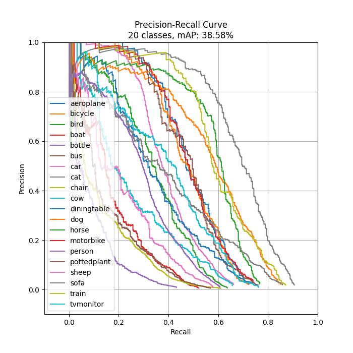
After learning about the mAP calculation from the above example, I will use this section to showcase an evaluation result of an SSD300-VGG16 model I trained on the PASCAL VOC 2007 trainval dataset (batch size = 32, epochs = 275 ≈ 42k iterations) and provide some of my opinions on how it can be improved. The evaluation is done on the test set of the same dataset. The number of detections produce by the SSD model is set to 200 (same as SSD paper) while the IOU threshold is set to 50% as in the PASCAL VOC challenge.
AI/ML
Trending AI/ML Article Identified & Digested via Granola by Ramsey Elbasheer; a Machine-Driven RSS Bot
via WordPress https://ramseyelbasheer.io/2021/06/26/implementing-single-shot-detector-ssd-in-keras-part-vi%e2%80%8a-%e2%80%8amodel-evaluation/


