Annotate dense point cloud data using SageMaker Ground Truth
Original Source Here
Autonomous vehicle companies typically use LiDAR sensors to generate a 3D understanding of the environment around their vehicles. For example, they mount a LiDAR sensor on their vehicles to continuously capture point-in-time snapshots of the surrounding 3D environment. The LiDAR sensor output is a sequence of 3D point cloud frames (the typical capture rate is 10 frames per second). Amazon SageMaker Ground Truth makes it easy to label objects in a single 3D frame or across a sequence of 3D point cloud frames for building machine learning (ML) training datasets. Ground Truth also supports sensor fusion of camera and LiDAR data with up to eight video camera inputs.
As LiDAR sensors become more accessible and cost-effective, customers are increasingly using point cloud data in new spaces like robotics, signal mapping, and augmented reality. Some new mobile devices even include LiDAR sensors, one of which supplied the data for this post! The growing availability of LiDAR sensors has increased interest in point cloud data for ML tasks, like 3D object detection and tracking, 3D segmentation, 3D object synthesis and reconstruction, and even using 3D data to validate 2D depth estimation.
Although dense point cloud data is rich in information (over 1 million point clouds), it’s challenging to label because labeling workstations often have limited memory, and graphics capabilities and annotators tend to be geographically distributed, which can increase latency. Although large numbers of points may be renderable in a labeler’s workstation, labeler throughput can be reduced due to rendering time when dealing with multi-million sized point clouds, greatly increasing labeling costs and reducing efficiency.
A way to reduce these costs and time is to convert point cloud labeling jobs into smaller, more easily rendered tasks that preserve most of the point cloud’s original information for annotation. We refer to these approaches broadly as downsampling, similar to downsampling in the signal processing domain. Like in the signal processing domain, point cloud downsampling approaches attempt to remove points while preserving the fidelity of the original point cloud. When annotating downsampled point clouds, you can use the output 3D cuboids for object tracking and object detection tasks directly for training or validation on the full-size point cloud with little to no impact on model performance while saving labeling time. For other modalities, like semantic segmentation, in which each point has its own label, you can use your downsampled labels to predict the labels on each point in the original point cloud, allowing you to perform a tradeoff between labeler cost (and therefore amount of labeled data) and a small amount of misclassifications of points in the full-size point cloud.
In this post, we walk through how to perform downsampling techniques to prepare your point cloud data for labeling, then demonstrate how to upsample your output labels to apply to your original full-size dataset using some in-sample inference with a simple ML model. To accomplish this, we use Ground Truth and Amazon SageMaker notebook instances to perform labeling and all preprocessing and postprocessing steps.
The data
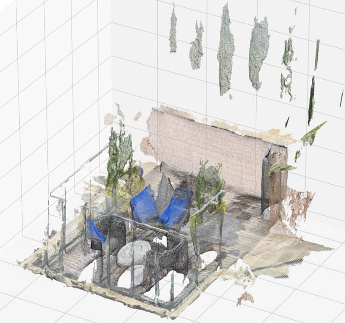
The data we use in this post is a scan of an apartment building rooftop generated using the 3D Scanner App on an iPhone12 Pro. The app allows you to use the built-in LiDAR scanners on mobile devices to scan a given area and export a point cloud file. In this case, the point cloud data is in xyzrgb format, an accepted format for a Ground Truth point cloud. For more information about the data types allowed in a Ground Truth point cloud, see Accepted Raw 3D Data Formats.
The following image shows our 3D scan.
Methods
We first walk through a few approaches to reduce dataset size for labeling point clouds: tiling, fixed step sample, and voxel mean. We demonstrate why downsampling techniques can increase your labeling throughput without significantly sacrificing annotation quality, and then we demonstrate how to use labels created on the downsampled point cloud and apply them to your original point cloud with an upsampling approach.
Downsampling approaches
Downsampling is taking your full-size dataset and either choosing a subset of points from it to label, or creating a representative set of new points that aren’t necessarily in the original dataset, but are close enough to allow labeling.
Tiling
One naive approach is to break your point cloud space into 3D cubes, otherwise known as voxels, of (for example) 500,000 points each that are labeled independently in parallel. This approach, called tiling, effectively reduces the scene size for labeling.
However, it can greatly increase labeling time and costs, because a typical 8-million-point scene may need to be broken up into over 16 sub-scenes. The large number of independent tasks that result from this method means more annotator time is spent on context switching between tasks, and workers may lose context when the scene is too small, resulting in mislabeled data.
Fixed step sample
An alternative approach is to select or create a reduced number of points by a linear subsample, called a fixed step sample. Let’s say you want to hit a target of 500,000 points (we have observed this is generally renderable on a consumer laptop—see Accepted Raw 3D Data Format), but you have a point cloud with 10 million points. You can calculate your step size as step = 10,000,000 / 500,000 = 20. After you have a step size, you can select every 20th point in your dataset, creating a new point cloud. If your point cloud data is of high enough density, labelers should still be able to make out any relevant features for labeling even though you may only have 1 point for every 20 in the original scene.
The downside of this approach is that not all points contribute to the final downsampled result, meaning that if a point is one of few important ones, but not part of the sample, your annotators may miss the feature entirely.
Voxel mean
An alternate form of downsampling that uses all points to generate a downsampled point cloud is to perform grid filtering. Grid filtering means you break the input space into regular 3D boxes (or voxels) across the point cloud and replace all points within a voxel with a single representative point (the average point, for example). The following diagram shows an example voxel red box.
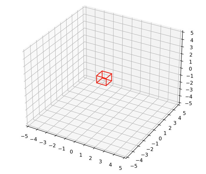
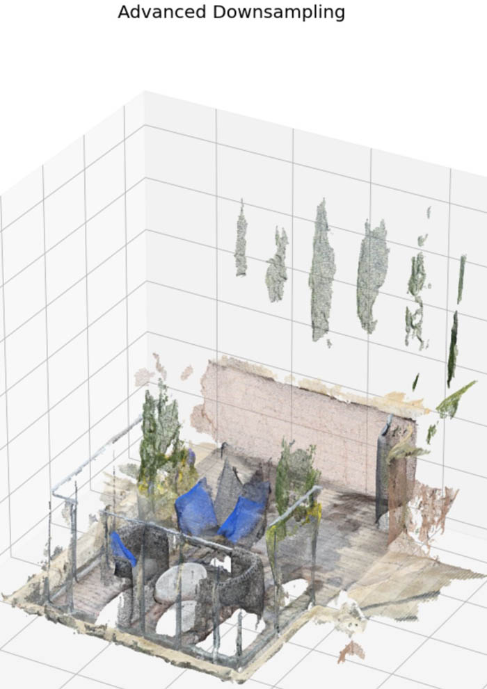
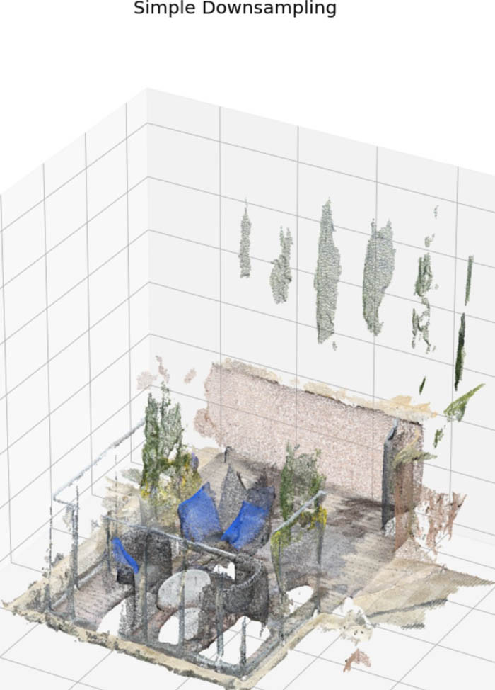
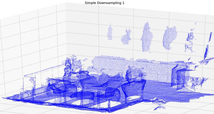
If no points exist from the input dataset within a given voxel, no point is added to the downsampled point cloud for that voxel. Grid filtering differs from a fixed step sample because you can use it to reduce noise and further tune it by adjusting the kernel size and averaging function to result in slightly different final point clouds. The following point clouds show the results of simple (fixed step sample) and advanced (voxel mean) downsampling. The point cloud downsampled using the advanced method is smoother, this is particularly noticeable when comparing the red brick wall in the back of both scenes.

Upsampling approach
After downsampling and labeling your data, you may want to see the labels produced on the smaller, downsampled point cloud projected onto the full-size point cloud, which we call upsampling. Object detection or tracking jobs don’t require post-processing to do this. Labels in the downsampled point cloud (like cuboids) are directly applicable to the larger point cloud because they’re defined in a world coordinate space shared by the full-size point cloud (x, y, z, height, width, length). These labels are minimally susceptible to very small errors along the boundaries of objects when a boundary point wasn’t in the downsampled dataset, but such occasional and minor errors are outweighed by the number of extra, correctly labeled points within the cuboid that can also be trained on.
For 3D point cloud semantic segmentation jobs, however, the labels aren’t directly applicable to the full-size dataset. We only have a subset of the labels, but we want to predict the rest of the full dataset labels based on this subset. To do this, we can use a simple K-Nearest Neighbors (K-NN) classifier with the already labeled points serving as the training set. K-NN is a simple supervised ML algorithm that predicts the label of a point using the “K” closest labeled points and a weighted vote. With K-NN, we can predict the point class of the rest of the unlabeled points in the full-size dataset based on the majority class of the three closest (by Euclidean distance) points. We can further refine this approach by varying the hyperparameters of a K-NN classifier, like the number of closest points to consider as well as the distance metric and weighting scheme of points.
After you map the sample labels to the full dataset, you can visualize tiles within the full-size dataset to see how well the upsampling strategy worked.
Now that we’ve reviewed the methods used in this post, we demonstrate these techniques in a SageMaker notebook on an example semantic segmentation point cloud scene.
Prerequisites
To walk through this solution, you need the following:
- An AWS account.
- A notebook AWS Identity and Access Management (IAM) role with the permissions required to complete this walkthrough. Your IAM role must have the following AWS managed policies attached:
AmazonS3FullAccessAmazonSageMakerFullAccess
- An Amazon Simple Storage Service (Amazon S3) bucket where the notebook artifacts (input data and labels) are stored.
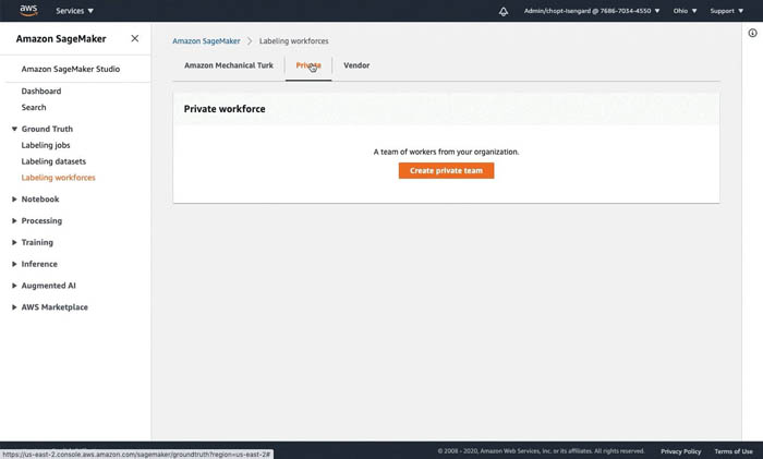
- A SageMaker work team. For this post, we use a private work team. You can create a work team on the SageMaker console.
Notebook setup
We use the notebook ground_truth_annotation_dense_point_cloud_tutorial.ipynb in the SageMaker Examples section of a notebook instance to demonstrate these downsampling and upsampling approaches. This notebook contains all code required to perform preprocessing, labeling, and postprocessing.
To access the notebook, complete the following steps:
- Create a notebook instance. You can use the instance type, ml.t2.xlarge, to launch the notebook instance. Please choose an instance with at least 16 GB of RAM.
- You need to use the notebook IAM role you created early. This role allows your notebook to upload your dataset to Amazon S3 and call the solution APIs.
- Open Jupyter Lab or Jupyter to access your notebook instance.
- In Jupyter, choose the SageMaker Examples In Jupyter Lab, choose the SageMaker icon.
- Choose Ground Truth Labeling Jobs and then choose the ipynb notebook.
- If you’re using Jupyter, choose Use to copy the notebook to your instance and run it. If you’re in Jupyter lab, choose Create a Copy.
Provide notebook inputs
First, we modify the notebook to add our private work team ARN and the bucket location we use to store our dataset as well as our labels.
Section 1: Retrieve the dataset and visualize the point cloud
We download our data by running Section 1 of our notebook, which downloads our dataset from Amazon S3 and loads the point cloud into our notebook instance. We download custom prepared data from an AWS owned bucket. An object called rooftop_12_49_41.xyz should be in the root of the S3 bucket. This data is a scan of an apartment building rooftop custom generated on a mobile device. In this case, the point cloud data is in xyzrgb format.
We can visualize our point cloud using the Matplotlib scatter3d function. The point cloud file contains all the correct points but isn’t rotated correctly. We can rotate the object around its axis by multiplying the point cloud by a rotation matrix. We can obtain a rotation matrix using scipy and specify the degree changes we want to make to each axis using the from_euler method:
!aws s3 cp s3://smgt-downsampling-us-east-1-322552456788/rooftop_12_49_41.xyz pointcloud.xyz

# Let's read our dataset into a numpy file
pc = np.loadtxt("pointcloud.xyz", delimiter=",")

print(f"Loaded points of shape {pc.shape}")

# playing with view of 3D scene

from scipy.spatial.transform import Rotation

def plot_pointcloud(pc, rot = [[30,90,60]], color=True, title="Simple Downsampling 1", figsize=(50,25), verbose=False):
    if rot:
        rot1 = Rotation.from_euler('zyx', [[30,90,60]], degrees=True)
        R1 = rot1.as_matrix()
        if verbose:
            print('Rotation matrix:','\n',R1)

        # matrix multiplication between our rotation matrix and pointcloud
        pc_show = np.matmul(R1, pc.copy()[:,:3].transpose() ).transpose()
        if color:
            try:
                rot_color1 = np.matmul(R1, pc.copy()[:,3:].transpose() ).transpose().squeeze()
            except:
                rot_color1 = np.matmul(R1, np.tile(pc.copy()[:,3],(3,1))).transpose().squeeze()
    else:
        pc_show = pc

    fig = plt.figure( figsize=figsize)
    ax = fig.add_subplot(111, projection="3d")
    ax.set_title(title, fontdict={'fontsize':20})
    if color:
        ax.scatter(pc_show[:,0], pc_show[:,1], pc_show[:,2], c=rot_color1[:,0], s=0.05)
    else:
        ax.scatter(pc_show[:,0], pc_show[:,1], pc_show[:,2], c='blue', s=0.05)

# rotate in z direction 30 degrees, y direction 90 degrees, and x direction 60 degrees
rot1 = Rotation.from_euler('zyx', [[30,90,60]], degrees=True)
print('Rotation matrix:','\n', rot1.as_matrix())

plot_pointcloud(pc, rot = [[30,90,60]], color=True, title="Full pointcloud", figsize=(50,30))
Section 2: Downsample the dataset
Next, we downsample the dataset to less than 500,000 points, which is an ideal number of points for visualizing and labeling. For more information, see the Point Cloud Resolution Limits in Accepted Raw 3D Data Formats. Then we plot the results of our downsampling by running Section 2.
As we discussed earlier, the simplest form of downsampling is to choose values using a fixed step size based on how large we want our resulting point cloud to be.
A more advanced approach is to break the input space into cubes, otherwise known as voxels, and choose a single point per box using an averaging function. A simple implementation of this is shown in the following code.
You can tune the target number of points and box size used to see the reduction in point cloud clarity as more aggressive downsampling is performed.
#Basic Approach
target_num_pts = 500_000
subsample = int(np.ceil(len(pc) / target_num_pts))
pc_downsample_simple = pc[::subsample]
print(f"We've subsampled to {len(pc_downsample_simple)} points")

#Advanced Approach
boxsize = 0.013 # 1.3 cm box size.
mins = pc[:,:3].min(axis=0)
maxes = pc[:,:3].max(axis=0)
volume = maxes - mins
num_boxes_per_axis = np.ceil(volume / boxsize).astype('int32').tolist()
num_boxes_per_axis.extend([1])

print(num_boxes_per_axis)

# For each voxel or "box", use the mean of the box to chose which points are in the box.
means, _, _ = scipy.stats.binned_statistic_dd(
    pc[:,:4],
    [pc[:,0], pc[:,1], pc[:,2], pc[:,3]],
    statistic="mean",
    bins=num_boxes_per_axis,
)
x_means = means[0,~np.isnan(means[0])].flatten()
y_means = means[1,~np.isnan(means[1])].flatten()
z_means = means[2,~np.isnan(means[2])].flatten()
c_means = means[3,~np.isnan(means[3])].flatten()
pc_downsample_adv = np.column_stack([x_means, y_means, z_means, c_means])
print(pc_downsample_adv.shape)
Section 3: Visualize the 3D rendering
We can visualize point clouds using a 3D scatter plot of the points. Although our point clouds have color, our transforms have different effects on color, so comparing them in a single color provides a better comparison. We can see that the advanced voxel mean method creates a smoother point cloud because averaging has a noise reduction effect. In the following code, we can look at our point clouds from two separate perspectives by multiplying our point clouds by different rotation matrices.
When you run Section 3 in the notebook, you also see a comparison of a linear step approach versus a box grid approach, specifically in how the box grid filter has a slight smoothing effect on the overall point cloud. This smoothing could be important depending on the noise level of your dataset. Modifying the grid filtering function from mean to median or some other averaging function can also improve the final point cloud clarity. Look carefully at the back wall of the simple (fixed step size) and advanced (voxel mean) downsampled examples, notice the smoothing effect the voxel mean method has compared to the fixed step size method.
rot1 = Rotation.from_euler('zyx', [[30,90,60]], degrees=True)
R1 = rot1.as_matrix()

simple_rot1 = pc_downsample_simple.copy()
simple_rot1 = np.matmul(R1, simple_rot1[:,:3].transpose() ).transpose()
advanced_rot1 = pc_downsample_adv.copy()
advanced_rot1 = np.matmul(R1, advanced_rot1[:,:3].transpose() ).transpose()

fig = plt.figure( figsize=(50, 30))
ax = fig.add_subplot(121, projection="3d")
ax.set_title("Simple Downsampling 1", fontdict={'fontsize':20})
ax.scatter(simple_rot1[:,0], simple_rot1[:,1], simple_rot1[:,2], c='blue', s=0.05)
ax = fig.add_subplot(122, projection="3d")
ax.set_title("Voxel Mean Downsampling 1", fontdict={'fontsize':20})
ax.scatter(advanced_rot1[:,0], advanced_rot1[:,1], advanced_rot1[:,2], c='blue', s=0.05)

# to look at any of the individual pointclouds or rotate the pointcloud, use the following function

plot_pointcloud(pc_downsample_adv, rot = [[30,90,60]], color=True, title="Advanced Downsampling", figsize=(50,30))

Section 4: Launch a Semantic Segmentation Job
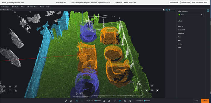
Run Section 4 in the notebook to take this point cloud and launch a Ground Truth point cloud semantic segmentation labeling job using it. These cells generate the required input manifest file and format the point cloud in a Ground Truth compatible representation.
To learn more about the input format of Ground Truth as it relates to point cloud data, see Input Data and Accepted Raw 3D Data Formats.
In this section, we also perform the labeling in the worker portal. We label a subset of the point cloud to have some annotations to perform upsampling with. When the job is complete, we load the annotations from Amazon S3 into a NumPy array for our postprocessing. The following is a screenshot from the Ground Truth point cloud semantic segmentation tool.
Section 5: Perform label upsampling
Now that we have the downsampled labels, we train a K-NN classifier from SKLearn to predict the full dataset labels by treating our annotated points as training data and performing inference on the remainder of the unlabeled points in our full-size point cloud.
You can tune the number of points used as well as the distance metric and weighting scheme to influence how label inference is performed. If you label a few tiles in the full-size dataset, you can use those labeled tiles as ground truth to evaluate the accuracy of the K-NN predictions. You can then use this accuracy metric for hyperparameter tuning of K-NN or to try different inference algorithms to reduce your number of misclassified points between object boundaries, resulting in the lowest possible in-sample error rate. See the following code:
# There's a lot of possibility to tune KNN further
# 1) Prevent classification of points far away from all other points (random unfiltered ground point)
# 2) Perform a non-uniform weighted vote
# 3) Tweak number of neighbors
knn = KNeighborsClassifier(n_neighbors=3)
print(f"Training on {len(pc_downsample_adv)} labeled points")
knn.fit(pc_downsample_adv[:,:3], annotations)

print(f"Upsampled to {len(pc)} labeled points")
annotations_full = knn.predict(pc[:,:3])
Section 6: Visualize the upsampled labels
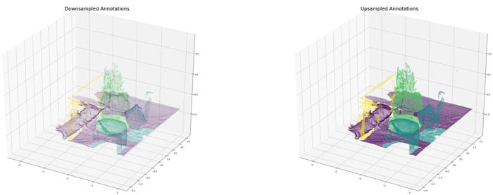
Now that we have performed upsampling of our labeled data, we can visualize a tile of the original full-size point cloud. We aren’t rendering all of the full-size point cloud because that may prevent our visualization tool from rendering. See the following code:
pc_downsample_annotated = np.column_stack((pc_downsample_adv[:,:3], annotations))
pc_annotated = np.column_stack((pc[:,:3], annotations_full))

labeled_area = pc_downsample_annotated[pc_downsample_annotated[:,3] != 255]
min_bounds = np.min(labeled_area, axis=0)
max_bounds = np.max(labeled_area, axis=0)

min_bounds = [-2, -2, -4.5, -1]
max_bounds = [2, 2, -1, 256]

def extract_tile(point_cloud, min_bounds, max_bounds):
    return point_cloud[
        (point_cloud[:,0] > min_bounds[0])
        & (point_cloud[:,1] > min_bounds[1])
        & (point_cloud[:,2] > min_bounds[2])
        & (point_cloud[:,0] < max_bounds[0])
        & (point_cloud[:,1] < max_bounds[1])
        & (point_cloud[:,2] < max_bounds[2])
    ]


tile_downsample_annotated = extract_tile(pc_downsample_annotated, min_bounds, max_bounds)
tile_annotated = extract_tile(pc_annotated, min_bounds, max_bounds)

rot1 = Rotation.from_euler('zyx', [[30,90,60]], degrees=True)
R1 = rot1.as_matrix()

down_rot = tile_downsample_annotated.copy()
down_rot = np.matmul(R1, down_rot[:,:3].transpose() ).transpose()
down_rot_color = np.matmul(R1, np.tile(tile_downsample_annotated.copy()[:,3],(3,1))).transpose().squeeze()

full_rot = tile_annotated.copy()
full_rot = np.matmul(R1, full_rot[:,:3].transpose() ).transpose()
full_rot_color = np.matmul(R1, np.tile(tile_annotated.copy()[:,3],(3,1))).transpose().squeeze()


fig = plt.figure(figsize=(50, 20))
ax = fig.add_subplot(121, projection="3d")
ax.set_title("Downsampled Annotations", fontdict={'fontsize':20})
ax.scatter(down_rot[:,0], down_rot[:,1], down_rot[:,2], c=down_rot_color[:,0], s=0.05)
ax = fig.add_subplot(122, projection="3d")
ax.set_title("Upsampled Annotations", fontdict={'fontsize':20})
ax.scatter(full_rot[:,0], full_rot[:,1], full_rot[:,2], c=full_rot_color[:,0], s=0.05)
Because our dataset is dense, we can visualize the upsampled labels within a tile to see the downsampled labels upsampled to the full-size point cloud. Although a small number of misclassifications may exist along boundary regions between objects, you also have many more correctly labeled points in the full-size point cloud than the initial point cloud, meaning your overall ML accuracy may improve.
Cleanup
Notebook instance: you have two options if you do not want to keep the created notebook instance running. If you would like to save it for later, you can stop rather than deleting it.
- To stop a notebook instance: click the Notebook instances link in the left pane of the SageMaker console home page. Next, click the Stop link under the ‘Actions’ column to the left of your notebook instance’s name. After the notebook instance is stopped, you can start it again by clicking the Start link. Keep in mind that if you stop rather than delete it, you will be charged for the storage associated with it.
- To delete a notebook instance: first stop it per the instruction above. Next, click the radio button next to your notebook instance, then select Delete from the Actions drop down menu.
Conclusion
Downsampling point clouds can be a viable method when preprocessing data for object detection and object tracking labeling. It can reduce labeling costs while still generating high-quality output labels, especially for 3D object detection and tracking tasks. In this post, we demonstrated how the downsampling method can affect the clarity of the point cloud for workers, and showed a few approaches that have tradeoffs based on the noise level of the dataset.
Finally, we showed that you can perform 3D point cloud semantic segmentation jobs on downsampled datasets and map the labels to the full-size point cloud through in-sample prediction. We accomplished this by training a classifier to do inference on the remaining full dataset size points, using the already labeled points as training data. This approach enables cost-effective labeling of highly dense point cloud scenes while still maintaining good overall label quality.
Test out this notebook with your own dense point cloud scenes in Ground Truth, try out new downsampling techniques, and even try new models beyond K-NN for final in-sample prediction to see if downsampling and upsampling techniques can reduce your labeling costs.
About the Authors
 Vidya Sagar Ravipati is a Deep Learning Architect at the Amazon ML Solutions Lab, where he leverages his vast experience in large-scale distributed systems and his passion for machine learning to help AWS customers across different industry verticals accelerate their AI and cloud adoption. Previously, he was a Machine Learning Engineer in Connectivity Services at Amazon who helped to build personalization and predictive maintenance platforms.
 Isaac Privitera is a Machine Learning Specialist Solutions Architect and helps customers design and build enterprise-grade computer vision solutions on AWS. Isaac has a background in using machine learning and accelerated computing for computer vision and signals analysis. Isaac also enjoys cooking, hiking, and keeping up with the latest advancements in machine learning in his spare time.
 Jeremy Feltracco is a Software Development Engineer with the Amazon ML Solutions Lab at Amazon Web Services. He uses his background in computer vision, robotics, and machine learning to help AWS customers accelerate their AI adoption.
AI/ML
Trending AI/ML Article Identified & Digested via Granola by Ramsey Elbasheer; a Machine-Driven RSS Bot
via WordPress https://ramseyelbasheer.io/2021/04/29/annotate-dense-point-cloud-data-using-sagemaker-ground-truth/