[Deep Learning]Sequence to Sequence Learning with Neural Networks Review (Seq2Seq)
Original Source Here
[Deep Learning]Sequence to Sequence Learning with Neural Networks Review (Seq2Seq)
# 대부분의 논문에서 소개하는 모델의 성능이 우수하게 나오기에, 성능에 대한 부분은 제외하였습니다.
✏️ 한글말로 풀어쓴 Seq2Seq 논문 (Please Speak in Korean!)
DNN(Deep Neural Network)은 기존의 ‘크기가 고정된 입력’에 대해서만 데이터를 처리할 수 있었습니다 . 대부분의 입력이 입력의 크기가 정해져 있지 않기 때문에 이러한 Sequential problem이 발생했습니다. Speech Recognition 과 Machine Translation이 대표적인 문제였는데, 이러한 단점을 보안하기 위해서 생긴것이 Sequence to Sequence입니다. 즉, 입력과 출력의 크기가 고정되어 있지 않아도 학습이 가능하게 만드는 것입니다.
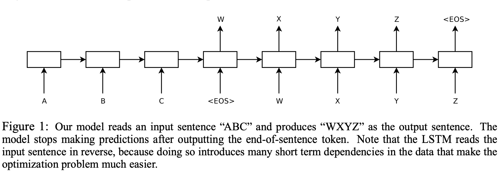
이 과정이 가능했던 것은 LSTM Encoder-decoder를 사용하여 길이에 성관없는 Input과 Output을 만들어냈다는 것입니다. 문장을 거꾸로 넣은 것이 더 성능이 좋았다는데 자세한 이유는 적혀져 있지 않습니다. (본인들도 모르는 듯 합니다.)
Encoder의 마지막 LSTM Layer Hidden State(알파벳C 가 들어가는 cell의 옆 화살표 부분)에서는 fixed-size vector로 Input Sequence의 정보가 합쳐져 있습니다. 이는 Encoding된 vector입니다. 다시 정리해보면, 임의의 길이를 가진 Input sequence를 fixed-size vector로 변환해주는 것이 Encoding 입니다.
RNN구조의 문제점은 input으로 무언가를 받으면 이전의 hidden state와 함께 현재의 hidden state가 계산되었고, 여기에 가중치가 곱해져서 Output을 만들어냈습니다. 여기서 문제가 발생합니다.
input이 들어가는 동시에 output이 만들어졌습니다. 그래서 계산 과정에서 target의 순서와 어떤 Source word가 어떤 Target word로 학습 돼야 하는지 제대로 이루어지지 않았습니다.
그래서 seq2seqt은 RNN을 통하여 Input sentence를 fixed-size vector로 만들었고 다른 RNN으로 output sequence를 만들어냈습니다.
더해서, RNN의 long-term-dependency문제를 해결하기위해 LSTM을 사용한 것입니다.
LSTM 뿐 아니라 GRU등의 RNN Cell들이 Encoder와 Decoder로 사용이 가능합니다. 이 논문에서는 LSTM을 사용하였습니다. 위의 조건부 확률에서
- x = input sequence
- y= output sequence
를 의미합니다. x가 주어졌을 때 y가 나올 확률을 높이는 쪽으로 학습이 진행되었습니다. p(y∣x)는 vocabulary의 모든 단어에 softmax를 적용한 것이다.
모든 문장의 끝에 token을 추가해서 문장이 끝임을 나타내었고 이를 같이 학습하였습니다. 그때부터 input sequence 에서 <EOS>라는 토큰이 나오게 되면 target sequence를 학습하는 식으로 진행하였고, output sequence에서 <EOS>가 나오면 그 때부터 generate하는 것을 중단하는 방식입니다.
요약해보면,
- 입력 문장과 출력문장을 위한 2개의 RNN cell을 사용하고
- 성능을 위해서 여러 개의 Deep LSTMs를 구성했습니다.
- 입력 문장의 단어 순서를 뒤집었는데 정배열보다 좋은 성능을 나타냈습니다.
🔥 Pytorch를 이용한 seq2seq 실습
처음에 요구되는 패키지를 불러옵니다. pytorch는 컴퓨터에 설치되어 있다고 가정합니다.
from __future__ import unicode_literals, print_function, division
from io import open
import unicodedata
import string
import re
import randomimport torch
import torch.nn as nn
from torch import optim
import torch.nn.functional as Fdevice = torch.device("cuda" if torch.cuda.is_available() else "cpu")
공식홈페이지에 나온 데이터를 사용하였습니다. 데이터는 영어-프랑스어 번역 쌍을 사용했습니다.
SOS_token = 0
EOS_token = 1
class Lang:
def __init__(self, name):
        self.name = name
        self.word2index = {}
        self.word2count = {}
        self.index2word = {0: "SOS", 1: "EOS"}
        self.n_words = 2  # SOS 와 EOS 포함    def addSentence(self, sentence):
for word in sentence.split(' '):
            self.addWord(word)    def addWord(self, word):
if word not in self.word2index:
            self.word2index[word] = self.n_words
            self.word2count[word] = 1
            self.index2word[self.n_words] = word
            self.n_words += 1
else:
            self.word2count[word] += 1
- One-Hot Encoding을 활용하여 그 단어 하나를 제외한 다른 단어들을 벡터 0으로 표현합니다. (Ex. 나는 배가 아파서 화장실에 갔다. ‘아파서’ = [0,0,1,0,0]
- <SOS>, <EOS> 시작 토큰과 종결 토큰을 달아줍니다.
- 나중에 모델에 넣기 위해서 단어의 index가 필요하기에 word2index와 색인으로 단어를 찾는 index2word 그리고 빈도수가 낮은 단어를 대체하는 데 사용하기 위해 word2count로 각 단어의 빈도수를 셀 수 있는 Class Lang을 생성합니다.
def unicodeToAscii(s):
return ''.join(
        c for c in unicodedata.normalize('NFD', s)
if unicodedata.category(c) != 'Mn'
    )
def normalizeString(s):
    s = unicodeToAscii(s.lower().strip())
    s = re.sub(r"([.!?])", r" \1", s)
    s = re.sub(r"[^a-zA-Z.!?]+", r" ", s)
return s
유니코드를 아스키코드로 변환해주고, 대문자to소문자 구분점을 지워주는 함수를 만듭니다.
def readLangs(lang1, lang2, reverse=False):
    print("Reading lines...")    # 파일을 읽고 줄로 분리
    lines = open('data/%s-%s.txt' % (lang1, lang2), encoding='utf-8').\
        read().strip().split('\n')    # 모든 줄을 쌍으로 분리하고 정규화
    pairs = [[normalizeString(s) for s in l.split('\t')] for l in lines]    # 쌍을 뒤집고, Lang 인스턴스 생성
if reverse:
        pairs = [list(reversed(p)) for p in pairs]
        input_lang = Lang(lang2)
        output_lang = Lang(lang1)
else:
        input_lang = Lang(lang1)
        output_lang = Lang(lang2)    return input_lang, output_lang, pairs
default는 영어->다른 언어이며, reverse = True로 할 경우, 다른 언어-> 영어 가 가능합니다.
MAX_LENGTH = 10eng_prefixes = (
    "i am ", "i m ",
    "he is", "he s ",
    "she is", "she s ",
    "you are", "you re ",
    "we are", "we re ",
    "they are", "they re "
)
def filterPair(p):
return len(p[0].split(' ')) < MAX_LENGTH and \
        len(p[1].split(' ')) < MAX_LENGTH and \
        p[1].startswith(eng_prefixes)
def filterPairs(pairs):
return [pair for pair in pairs if filterPair(pair)]
짧고 간단한 문장으로 데이터 셋을 정리할 것이며 이곳에는 종류 문장 부호가 포함됩니다.
input_lang, output_lang, pairs = readLangs(lang1, lang2, reverse)
    print("Read %s sentence pairs" % len(pairs))
    pairs = filterPairs(pairs)
    print("Trimmed to %s sentence pairs" % len(pairs))
    print("Counting words...")
for pair in pairs:
        input_lang.addSentence(pair[0])
        output_lang.addSentence(pair[1])
    print("Counted words:")
    print(input_lang.name, input_lang.n_words)
    print(output_lang.name, output_lang.n_words)
return input_lang, output_lang, pairs
input_lang, output_lang, pairs = prepareData('eng', 'fra', True)
print(random.choice(pairs))
텍스트 파일을 읽기 -> 줄로 분리하기 -> pairs로 분리하기
위의 과정을 걸친뒤 텍스트를 정규화하고 길이와 내용으로 필터링을 진행합니다. 그리고 pair를 이룬 문장들로 단어 리스트를 생성합니다. 이제 준비 과정은 끝났습니다.
## Encoder
모든 input sequence에 대해서 Encoder는 vector +previous hidden state를 출력하고 다음 입력 단어를 위해 그 hidden state를 사용합니다.
lass EncoderRNN(nn.Module):
def __init__(self, input_size, hidden_size):
        super(EncoderRNN, self).__init__()
        self.hidden_size = hidden_size        self.embedding = nn.Embedding(input_size, hidden_size)
        self.gru = nn.GRU(hidden_size, hidden_size)    def forward(self, input, hidden):
        embedded = self.embedding(input).view(1, 1, -1)
        output = embedded
        output, hidden = self.gru(output, hidden)
return output, hidden    def initHidden(self):
return torch.zeros(1, 1, self.hidden_size, device=device)
## Decoder
Encoder의 마지막 출력만을 이용하며, 이 출력은 전체 sequence에서 문맥을 encoding하기 때문에 context vector(문맥 벡터)로 불립니다. 이 context vector는 decoder의 초기 hidden state로 사용됩니다. decoding은 매 단계에서 decoder에게 input token과 hidden state가 주어집니다.
- 초기 input token은 <SOS> 토큰(start of string)이며
- 첫 hidden state는 encoder의 마지막 hidden state인 context vector입니다.
class DecoderRNN(nn.Module):
def __init__(self, hidden_size, output_size):
        super(DecoderRNN, self).__init__()
        self.hidden_size = hidden_size        self.embedding = nn.Embedding(output_size, hidden_size)
        self.gru = nn.GRU(hidden_size, hidden_size)
        self.out = nn.Linear(hidden_size, output_size)
        self.softmax = nn.LogSoftmax(dim=1)    def forward(self, input, hidden):
        output = self.embedding(input).view(1, 1, -1)
        output = F.relu(output)
        output, hidden = self.gru(output, hidden)
        output = self.softmax(self.out(output[0]))
return output, hidden    def initHidden(self):
return torch.zeros(1, 1, self.hidden_size, device=device)
## Attention Decoder
context vector만 encoder와 decoder사이로 전달이 된다면, 단일 vector가 전체 문장을 encoding 해야하는 문제가 생긴다. Attention Mechanism을 사용하여 Decoder가 자기 출력의 모든 단계에서 인코더 출력의 다른 부분에 집중 할 수 있게 한다. 즉, 디코더의 특정 time-step의 output이 인코더의 모든 time-step의 output 중 어떤 time-step과 가장 연관이 있는가가 주요 task입니다.
- 이 부분은 블로그의 추후 뒷글에서 설명할 예정입니다. link
class AttnDecoderRNN(nn.Module):
def __init__(self, hidden_size, output_size, dropout_p=0.1, max_length=MAX_LENGTH):
        super(AttnDecoderRNN, self).__init__()
        self.hidden_size = hidden_size
        self.output_size = output_size
        self.dropout_p = dropout_p
        self.max_length = max_length        self.embedding = nn.Embedding(self.output_size, self.hidden_size)
        self.attn = nn.Linear(self.hidden_size * 2, self.max_length)
        self.attn_combine = nn.Linear(self.hidden_size * 2, self.hidden_size)
        self.dropout = nn.Dropout(self.dropout_p)
        self.gru = nn.GRU(self.hidden_size, self.hidden_size)
        self.out = nn.Linear(self.hidden_size, self.output_size)    def forward(self, input, hidden, encoder_outputs):
        embedded = self.embedding(input).view(1, 1, -1)
        embedded = self.dropout(embedded)        attn_weights = F.softmax(
            self.attn(torch.cat((embedded[0], hidden[0]), 1)), dim=1)
        attn_applied = torch.bmm(attn_weights.unsqueeze(0),
                                 encoder_outputs.unsqueeze(0))        output = torch.cat((embedded[0], attn_applied[0]), 1)
        output = self.attn_combine(output).unsqueeze(0)        output = F.relu(output)
        output, hidden = self.gru(output, hidden)        output = F.log_softmax(self.out(output[0]), dim=1)
return output, hidden, attn_weights    def initHidden(self):
return torch.zeros(1, 1, self.hidden_size, device=device)
## Training dataset
학습을 위해서 input sentence 주소와 target sentence주소를 지정해 줘야 합니다. 이 벡터들을 생성하는 동안 이 두 sequence에 <EOS> 토큰을 추가해줍니다.
def indexesFromSentence(lang, sentence):
return [lang.word2index[word] for word in sentence.split(' ')]
def tensorFromSentence(lang, sentence):
    indexes = indexesFromSentence(lang, sentence)
    indexes.append(EOS_token)
return torch.tensor(indexes, dtype=torch.long, device=device).view(-1, 1)
def tensorsFromPair(pair):
    input_tensor = tensorFromSentence(input_lang, pair[0])
    target_tensor = tensorFromSentence(output_lang, pair[1])
return (input_tensor, target_tensor)
## Training the model
학습을 위해 encoder에 input sentence를 넣고 모든 출력과 hidden state를 추적합니다. 그런 후 decoder에 첫 번째 입력으로 “<SOS>token과 encoder의 latest hidden state가” 첫 번째 hidden state로 제공됩니다.
Teacher forcing ratio는 next input으로 decoder의 예측을 사용하는 것이 아니라 실제 target 출력을 다음 입력으로 사용합니다. 이를 사용하면 결과가 빨리출력되지만, 학습된 모델이 불안정성을 보일 수 있습니다.
teacher_forcing_ratio = 0.5
def train(input_tensor, target_tensor, encoder, decoder, encoder_optimizer, decoder_optimizer, criterion, max_length=MAX_LENGTH):
    encoder_hidden = encoder.initHidden()    encoder_optimizer.zero_grad()
    decoder_optimizer.zero_grad()    input_length = input_tensor.size(0)
    target_length = target_tensor.size(0)    encoder_outputs = torch.zeros(max_length, encoder.hidden_size, device=device)    loss = 0    for ei in range(input_length):
        encoder_output, encoder_hidden = encoder(
            input_tensor[ei], encoder_hidden)
        encoder_outputs[ei] = encoder_output[0, 0]    decoder_input = torch.tensor([[SOS_token]], device=device)    decoder_hidden = encoder_hidden    use_teacher_forcing = True if random.random() < teacher_forcing_ratio else False    if use_teacher_forcing:
# Teacher forcing 포함: 목표를 다음 입력으로 전달
for di in range(target_length):
            decoder_output, decoder_hidden, decoder_attention = decoder(
                decoder_input, decoder_hidden, encoder_outputs)
            loss += criterion(decoder_output, target_tensor[di])
            decoder_input = target_tensor[di]  # Teacher forcing    else:
# Teacher forcing 미포함: 자신의 예측을 다음 입력으로 사용
for di in range(target_length):
            decoder_output, decoder_hidden, decoder_attention = decoder(
                decoder_input, decoder_hidden, encoder_outputs)
            topv, topi = decoder_output.topk(1)
            decoder_input = topi.squeeze().detach()  # 입력으로 사용할 부분을 히스토리에서 분리            loss += criterion(decoder_output, target_tensor[di])
if decoder_input.item() == EOS_token:
break    loss.backward()    encoder_optimizer.step()
    decoder_optimizer.step()    return loss.item() / target_length
## 모델의 학습 진행률을 보여주는 함수입니다.
import time
import math
def asMinutes(s):
    m = math.floor(s / 60)
    s -= m * 60
return '%dm %ds' % (m, s)
def timeSince(since, percent):
    now = time.time()
    s = now - since
    es = s / (percent)
    rs = es - s
return '%s (- %s)' % (asMinutes(s), asMinutes(rs))
## 전체 학습 과정
def trainIters(encoder, decoder, n_iters, print_every=1000, plot_every=100, learning_rate=0.01):
    start = time.time()
    plot_losses = []
    print_loss_total = 0  # print_every 마다 초기화
    plot_loss_total = 0  # plot_every 마다 초기화    encoder_optimizer = optim.SGD(encoder.parameters(), lr=learning_rate)
    decoder_optimizer = optim.SGD(decoder.parameters(), lr=learning_rate)
    training_pairs = [tensorsFromPair(random.choice(pairs))
for i in range(n_iters)]
    criterion = nn.NLLLoss()    for iter in range(1, n_iters + 1):
        training_pair = training_pairs[iter - 1]
        input_tensor = training_pair[0]
        target_tensor = training_pair[1]        loss = train(input_tensor, target_tensor, encoder,
                     decoder, encoder_optimizer, decoder_optimizer, criterion)
        print_loss_total += loss
        plot_loss_total += loss        if iter % print_every == 0:
            print_loss_avg = print_loss_total / print_every
            print_loss_total = 0
            print('%s (%d %d%%) %.4f' % (timeSince(start, iter / n_iters),
                                         iter, iter / n_iters * 100, print_loss_avg))        if iter % plot_every == 0:
            plot_loss_avg = plot_loss_total / plot_every
            plot_losses.append(plot_loss_avg)
            plot_loss_total = 0    showPlot(plot_losses)
- 타이머 함수로 시작을 하고
- optimizer와 criterion을 초기화 해줍니다.
- 그리고 학습 pairs를 만들고
- plot of loss 구축을 위해 loss 값을 모읍니다.
그 후 진행률과 평균 loss를 계속해서 출력합니다.
## Result to plot
import matplotlib.pyplot as plt
plt.switch_backend('agg')
import matplotlib.ticker as ticker
import numpy as np
def showPlot(points):
    plt.figure()
    fig, ax = plt.subplots()
# 주기적인 간격에 이 locator가 tick을 설정
    loc = ticker.MultipleLocator(base=0.2)
    ax.yaxis.set_major_locator(loc)
    plt.plot(points)
mataplotlib으로 학습 도중에 손실된 값 plot_losses를 배열을 사용해서 도식화 해줍니다.
## Evaluation
평가는 target task가 없기 때문에 그냥 단순하게각 단계에서 decoder의 예측을 target task로 합니다. 과정은 training과 비슷합니다. 즉, decoder가 word를 예측할 때마다 그것을 output string에 더해주고 <EOS>토큰이 나올때 멈춰줍니다.추가로, decoder의 attention 또한 도식화를 위해 저장해 줍니다.
def evaluate(encoder, decoder, sentence, max_length=MAX_LENGTH):
with torch.no_grad():
        input_tensor = tensorFromSentence(input_lang, sentence)
        input_length = input_tensor.size()[0]
        encoder_hidden = encoder.initHidden()        encoder_outputs = torch.zeros(max_length, encoder.hidden_size, device=device)        for ei in range(input_length):
            encoder_output, encoder_hidden = encoder(input_tensor[ei],
                                                     encoder_hidden)
            encoder_outputs[ei] += encoder_output[0, 0]        decoder_input = torch.tensor([[SOS_token]], device=device)  # SOS        decoder_hidden = encoder_hidden        decoded_words = []
        decoder_attentions = torch.zeros(max_length, max_length)        for di in range(max_length):
            decoder_output, decoder_hidden, decoder_attention = decoder(
                decoder_input, decoder_hidden, encoder_outputs)
            decoder_attentions[di] = decoder_attention.data
            topv, topi = decoder_output.data.topk(1)
if topi.item() == EOS_token:
                decoded_words.append('<EOS>')
break
else:
                decoded_words.append(output_lang.index2word[topi.item()])            decoder_input = topi.squeeze().detach()        return decoded_words, decoder_attentions[:di + 1]
# Training and Evaluating
실제 학습과 평가가 이제 이루어질 것입니다. 맥북 기준으로 40분 걸린다고 나와있는데 나는 1시간넘게 결과가 안나왔습니다.
hidden_size = 256
encoder1 = EncoderRNN(input_lang.n_words, hidden_size).to(device)
attn_decoder1 = AttnDecoderRNN(hidden_size, output_lang.n_words, dropout_p=0.1).to(device)trainIters(encoder1, attn_decoder1, 75000, print_every=5000)
결과는 아래와 같습니다.
Out:
1m 39s (- 23m 17s) (5000 6%) 2.8399
3m 12s (- 20m 53s) (10000 13%) 2.2540
4m 48s (- 19m 12s) (15000 20%) 1.9613
6m 22s (- 17m 32s) (20000 26%) 1.6996
7m 56s (- 15m 53s) (25000 33%) 1.5200
9m 30s (- 14m 16s) (30000 40%) 1.3468
11m 3s (- 12m 38s) (35000 46%) 1.2412
12m 35s (- 11m 0s) (40000 53%) 1.0762
14m 8s (- 9m 25s) (45000 60%) 1.0066
15m 40s (- 7m 50s) (50000 66%) 0.8932
17m 12s (- 6m 15s) (55000 73%) 0.8285
18m 45s (- 4m 41s) (60000 80%) 0.7348
20m 19s (- 3m 7s) (65000 86%) 0.6596
21m 52s (- 1m 33s) (70000 93%) 0.6180
23m 25s (- 0m 0s) (75000 100%) 0.5659
### Visualizing Attention
- 사실상 attention은 아주 중요하고 seq2seq 설명 부분이라 넣을지 말지 고민했으나 그냥 넣었습니다. 초기 모델에서는 attention이라는 개념보다는 align이라는 개념으로 많이 소개 되었습니다. 자세한 설명은 우리 블로그의 Attention 파트에서 더 읽어보면 좋습니다.
attention을 사용한 이유에 대한 찬양이 나옵니다.
“ A useful property of the attention mechanism is its highly interpretable outputs. Because it is used to weight specific encoder outputs of the input sequence, we can imagine looking where the network is focused most at each time step.”
attention에 대한 도식화는 간단한 코드로 구현 가능합니다.
output_words, attentions = evaluate(
    encoder1, attn_decoder1, "je suis trop froid .")
plt.matshow(attentions.numpy())
AI/ML
Trending AI/ML Article Identified & Digested via Granola by Ramsey Elbasheer; a Machine-Driven RSS Bot
via WordPress https://ramseyelbasheer.io/2021/03/11/deep-learningsequence-to-sequence-learning-with-neural-networks-review-seq2seq/


