Transformers in Pytorch from scratch for NLP Beginners
Original Source Here
2/ The Transformer, a sequential data encoder
The Transformer is an encoder
Now that we have our input, it’s time to put it in a model!
Before going into the details, let’s just understand what transformers truly are. Transformers aren’t translators, transformers aren’t classifiers, transformers aren’t chatbots and transformers aren’t search engines.
The Transformer is mainly an encoder architecture.
The original transformer is an encoder-decoder architecture but let’s just say that this is a special case of transformer.
What it means is that for each representation in the input, you’ll have a representation in the output. And we can even further simplify, if the input is of dimension seq_len * embed_size, the output can be of dimension seq_len * embed_size.
The goal of the encoder will not be to append information, but to process the original embedding in another embedding of the same size, but this time which takes into account the whole sentence. The context.
You could change the size, you could append information, but that’s not necessary for things to work.
Language Models
Now above that encoder, you can put another model which is a Language Model. This language model takes the output of the transformer and do the task you need (for example, translation, which is a “next word classification” task). Chatbots also are close to “next word classification” models. POS tagging is just a classification task on a set of tags etc.
That’s the language model:
Input => Transformer => Language Model => Output
But we’ll get back to that later.
How do we re-build the idea of transformers from scratch?
Why Transformers?
Ok, my input is of shape (seq_len, embed_size). For each word I have a vector. Now what?
I’ll start by just giving some ideas.
1st idea: for each word, I take its vector, I concatenate all vectors of all other words in one big vector, I concatenate both and I put that as the input of a linear layer + relu multiple times. New input shape: (1, seq_len*embed_size)
Well… it’s not efficient. For the first vector of the current word, there’s no problem. But for the rest, the concatenation makes it so that even if the 1st value of the second word and the 1st value of the third word should be processed the same way, they won’t be. They should because in another sentence, the second word could be in place of the third word and we shouldn’t have to retrain parameters just because of that (it’s not a new word, just a new position, positional embeddings already encode the information we need).
Moreover, we can’t process larger sentences this way.
2nd idea: Let’s think of something else… well then we could process words one by one, from the left to the right having a constant size output and accumulate information as we read each word individually… yeah no ok that’s recurrent networks.
3rd idea: We could also use convolutional networks… and process our (seq_len, embed_size) matrix with multiple 1d convolutions… that’s how we did it before recurrent networks…we have to go forward.
4th idea: The first idea wasn’t that bad, we just need to have the same computations with the word we’re reading whatever the position of the other word is… well in this case, I can just use the current word embedding of shape (embed_size), the other word embedding of shape (embed_size), concatenate both (1 * [2*embed_size]), do a linear layer, and that’s it, I do that for each word pair. Yay that’s easy … … … No.
Of course that’s not how they did it because the expressiveness of such model would be quite low and you’ll get why.
Attention mechanism
But if you thought of doing that. You got the idea. We’re going to process words two by two. The first idea of Transformers is to turn each word embedding into three word embeddings. Why? Because using intermediate representations allows to do a bigger range of computations. You can do computations with an embedding without losing the original information in another embedding.
- For the first representation, the model will read the word as the main word being processed, the query.
- For the second representation, the model will read the word as the word being compared to the main processed word, the key.
- For the third representation, the model will read the word as a way to evaluate what information it should keep from that word to build the final representation of the main word.
I have a word (its embedding), I can use it as the main word being processed, I can use it as a word being processed with a main word, and I can use it as a way to value how much this other word should influence the new representation of the main word.
Three representations:
- The query is the main representation of the word for which we’re building a new representation (the main word)
- The key is the representation of all words when these words are being compared with a main word
- The value is the representation of all words — including the main word — we use to produce the final embedding
The comparison of the i-th “query” and the j-th “key” will produce a scalar, which is here to indicate how important the “value” of the j-th word is compared to other “values”. This is used to produce the new embedding of the i-th word.
For the i-th word, we compute the j-th scalar which weight the j-th value vector in the weighted sum of all value vectors. This weighted sum is the contextualized representation of the i-th word.
The maths
How do we create a new vector based on another in deep learning? Well if we want a vector of size M based on an input of size N, we just multiply the input by an (N,M) trainable matrix. (1,N) with (N,M) gives (1,M). In Pytorch, that’s nn.Linear (biases aren’t always required).
Ok, now what? Well we’re going to mathematically do what “compared to other words” means for transformers. We have q,k,v as input, and we want to produce one output that contains the information: what does this word mean when compared to all other words?
This is represented like that in the original “Attention is all you need” paper:
But a better way to understand the computations is by reading this :
For each word, the attention layer returns one vector z which means: “this is what this word means compared to all others”.
With seq_len = 20 and embed_size = 128, the input is of shape (20, 128). The attention layer outputs one vector for each word. q, k and v have the same shape: (20, 128). Keeping the same embed_size for q, k, v is easier for future computations but not necessry.
We do q ∙ k.T, shapes are (20, 128) dot (128, 20), we get one score for each two words in a matrix of shape (20,20). We scale that score (just for numerical stability, big values aren’t nice in deep learning) (20,20), we apply a softmax of all scores corresponding to a word (20,20), which means that all scores now sum to one. We do a weighted sum of all value vectors with the scores as weights, for each main word (20, 128).
So, v is of shape (20, 128) . Each vector v of each word will contribute to the output for each word. For the 1st word, we will read the 1st 20 values in our (20, 20) matrix, and we will do a weighted sum of these 20 values with the 20 vectors v, giving one (1, 128) embedding representing our 1st word put in context. We do the same for the 2nd word etc.
The context comes from all the other value vectors.
Why softmax? Well that’s the point of many attention algorithms, you give more weight to the most important element. The interaction between the first word and the last word aren’t probably as relevant as the interaction between the first word and the second word. With softmax, a low score will result in x being close to 0, and the fact that it sums to 1 helps in keeping the same scale of values even for relevant vectors. Otherwise one sum could give an embedding with values around +/-100 and another one could give values around +/-2. Again, in deep learning we don’t really like that. Small variations, small values: nice. Big possible variations, big values: harder to process.
Two last things: A mask and dropout. A mask because sometimes you know that a word shouldn’t have an influence on other words. That’s the case when you’re padding a short sentence of length 12 to have a length of 20 for a batch, you’ll want to ignore the influence of pads. And that’s also the case when you’re translating words sequentially and you don’t want future words to influence previous ones (that’s mostly for an encoder-decoder architecture).
And dropout for regularization, it helps the model to distribute the information consistently, it can’t focus on only one way to pass the information because this way is going to be randomly zero-ed out sometimes.
…
…Guess what?
That was the hardest part of the transformer architecture.
Let’s get back to what we were trying to do. For each word we wanted to create a representation that takes into account all other words. We did it!
Attention layer ✔️
Transformer modules
Now, the rest is just here to enhance computations.
- A transformer is a stack of encoders. t =[enc1, enc2 …]
- An encoder is composed of one MultiHeadAttention and one FeedForward layer. enc1 = [mha, ff]
- And MultiHeadAttention is composed of the Attention mechanism and extra tricks for a more efficient processing. mha = [attention]
t = attention, ff, attention, ff, attention, ff etc..
MultiHeadAttention Layer (MHA
We did one attention. Transformers use multiple attention simultaneously. We call that “heads”. If a transformer uses 8 heads, it’ll first cut the embedding (128) into a tensor of shape (8 heads, 16 smaller_embed_size) (128/8 = 16). If you have a sequence of length 20, the result is of shape (20, 8, 16). If you have a batch of size 128, the result is of shape (128, 20, 8, 16).
For easier computations, it’ll swap the 2nd and 3rd dimensions. For example, if we want to compute the score = q ∙ k.T for the attention layer. The shape of q is now (128, 8, 20, 16), k.T is of shape (128, 8, 16, 20). The score is of shape (128, 8, 20, 20). 8 heads, 8 attention maps.
Each head gives an attention map of (20,20) and each head ends with a vector of size 16, we concatenate the attention for 8 heads, and we get our embedding of size 128. It allows the model to learn multiple attention maps at the same time such that there isn’t necessary one word that’ll always have the biggest influence, each head uses softmax, giving 8 “smoothed” possibilities. “Smoothed” because it’s not always binary, one head could make softmax give a score of 0.45 for two words and make all the others close to 0, even if in general it focuses on one word.
We use a final linear layer to allow the model to mix these 8 concatenated representations into an uniform representation.
- Attention ✔️
- MultiHeadAttention✔️
- FeedForward ❌
FeedForward Layer (FF)
This is just the non-linearity layer. It takes the output of the MHA as an input.
It’s quite basic, for each embedding of shape (128), you multiply it by a trainable matrix of shape (128, 512), we’re using nn.Linear. It gives you a vector of size 512. You apply dropout, relu, whatever you want. And you scale back from 512 to 128 with another trainable matrix.
It is “applied to each position separately and identically”, says the original Transformer paper. It’s a way to re-process the representation coming out of the MHA with a non-linearity.
512 is the “inner feedforward size”. BERT takes that as 4 *embed_size. 4 * 128 = 512.
- Attention ✔️
- MultiHeadAttention✔️
- FeedForward ✔️
- Encoder ❌
Encoder Layer
The encoder is just a MHA followed by a FF.
Fun fact, the connections are residual. Not that it really changes anything to what we saw, it’s just nice to know that the algorithm doesn’t completely change the raw embedding we used but instead it adds what we computed to it. It learns to change the original representation instead of re-creating a new one.
But remember, because we’re training (almost) everything, all parameters will adapt suct that the sum makes sense. Residual connections are nice because they allow you to “enhance” an existing representation instead of creating a new one. And if your model contains residual connections, it’ll learn to gather information in the original representation.
It also adds some normalization (yes we still need that). But that’s not batch normalization because it has not been proven to be very efficient for transformers.
This time it’s Layer Normalization. It’s really easy:
- Batch norm: we have 100 objects with 10 values, we normalize 10 times across 100 objects
- Layer norm: we have 100 objects with 10 values, we normalize 100 times across 10 values
Batch norm is nice because it allows to indirectly compare representations between different objects but I guess we don’t need that in such architecture where we’re permanently comparing some representations with others.
Enough talking:
Basically: norm => mha => dropout => res add => norm => ff => dropout => res add
Transformer
The transformer is just a set of encoders.
That’s it! The final layer is a linear layer to implement the language model but a task-agnostic transformer network doesn’t need this. You can also see how we define embeddings. The input of the model is a list of integers (exp:[2,8,6,8,9]) corresponding to words (exo: [“red”, “and”, “blue”, “and”, “yellow”]). nn.Embeddings knows how to process that as indexes for its big (n_vocab, embed_size) matrix.
Now you know how to make a real Transformer.
PS: I checked my implementation with nn.Transformer from Pytorch and other implementations. I don’t guarantee everything but the number of parameters checks out with the right hyperparameters.
3/ The Language Model, the Task and the Dataset
To check that our model works, we need a task. I could take a supervised training dataset from Universal Dependencies or others.
But that’s boring, let’s do unsupervised training! We just need sentences, no labels! BERT doesn’t really define a new architecture, it mostly defines tasks that are new for transformers.
BERT does two tasks, first it defines an unmasking task, they call that a “masked language model” objective. It means that from a sentence of 20 words, it’ll remove 4 (for example) random words, and then it’ll ask the model to predict these 4 words based on all other words.
And BERT also does a next sentence prediction task. The idea is also simple. In a corpus with many sentences that follow each others, it’ll predict if the next sentence truly is the next sentence, and it’ll randomly change the next sentence with a random sentence. BERT will also add a sentence embedding corresponding to the relative sentence position (1st or 2nd).
BORING. We’re not doing that.
Let’s just keep it easy, we’re using word embeddings and positional embedding, and we’ll just do the masked words prediction task. We already talked about embeddings, let’s see how we mask words.
I can talk about that while presenting the dataset:
I initialize the dataset with all sentences preloaded (you can’t do that when you have 100 billion sentences), the vocabulary and the sequence length we want for making a batch.
We add special tags that will be used to replace some words. Mainly we have a tag for “out of vocabulary” words, which is very useful in order to know how to process a word we don’t know (that isn’t in the vocab). We have an <ignore> tag which is just here to tell the loss to ignore the prediction for non-masked words (we only want the loss for masked words). And we have a <mask> tag which is here so that we can replace the original word embedding with an universal “masked” embedding.
During training, we call __getitem__. We fetch the already tokenized sentence. We replace words by their assignated number in the vocab or by the number of the <out of vocabulary> tag. We ensure that the sequence has the good length and then we randomly mask words (15% chance) in the sentence.
If the word is masked, the input has the id of <mask> and the output has the id of the word (that the final linear layer of our model will try to predict). If the word isn’t masked, the input has the id of the word, and the output has the id of <ignore>, …which will be ignored by the loss.
The language model (which is represented by a Linear layer at the end of the Transformer model), will predict a score for each word of the vocab, so it’s a quite big layer with a trainable matrix of shape (128, 40000). (1, 128) dot (128, 40000) gives (1, 40000). You take the argmax and it gives the id of the word in the vocabulary. If the model did right, the argmax of that final layer corresponds to the id of the masked word.
Of course the unmasking task wasn’t just that in the BERT paper.
BERT masks words with a probability of 15%, but when a word is masked, 80% of the time it uses <mask>, 10% of the time it uses the original word and 10% of the time it uses a random word.
I’m not doing that for better readability.
4/ The Optimizer and the Loss
Fun fact, when you want to train word embeddings, some optimizers work, and others really don’t.
People often use SGD, but Adam can also work with some regularizations.
I tried RAdam, it completely failed to learn word embeddings on my setup.
The loss is CrossEntropy. It does a softmax such that the scores the layer attributes for each word prediction sum to one (like probabilities) and then we apply a negative log likelihood. That’s the usual way to do multi-class classification.
The loss ignores the prediction associated with the non-masked words thanks to the <ignore> tag we put as the label to predict for these words.
5/ Results
Finally! I won’t go into the details for the rest of the code. It’s one loop with comments. We get the batch, get the output of the model, put everything in the right shape for cross entropy and backpropagate.
How can we see if it worked?
Well, if the model was able to extract useful information, it should have been able to create meaningful embeddings.
How could we see that? … We’re going to use projector.tensorflow.org. This project allows to visualize embeddings. It’s quite simple, for each line of a file, we put the 128 values of the corresponding word separated with a tab \t.
Then we go to “Load” in projector.tensorflow.org. The first TSV files is values.tsv, it contains the vectors, and the second file contains the associated words.
We only take the first 3000 words because the web implementation of t-SNE can be quite slow to compute when you have too much words (you can take the first 1000 words if your computer doesn’t follow).
The algorithm applies a PCA by default. It’s already a way to visualize the information, but we’re going to use t-SNE which is a pretty great dimension-reduction algorithm for embeddings. It is made such that embeddings that are close in the original space stay close in the projected space. The original space is in dimension 128 (hard to understand for our 3D accustomed human eyes). We want a 3D/2D out space.
We just need to click T-SNE (bottom left), and the algorithm will do the computations. There’s a button to swap between 3D and 2D (I recommend 2D). You can pause when you have something that pleases you.
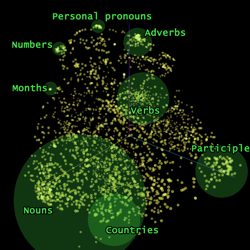
What you will want is something like that:
Clusters. Each cluster contains a bunch of words which are close by what they mean. More precisely these words are made to be interchangeable because these are the words the model needed to put close to make the task we were asking it easier.
The model couldn’t reduce the loss if it had to learn a complete different meaning for two close embeddings, so being able to reduce the loss means that the algorithm has to make two words that could be put in the same place close in the space of embeddings. The algorithm can do that because it can compute how to change an embedding to reduce the error thanks to backpropagation.
/!\ Disclaimer: you don’t need transformers to produce pretrained word embeddings. Transformers are a way to produce word embeddings but most importantly they aim at improving context modeling with a whole (pretrained embedding+transformer) model. So just vizualizing or using pretrained word embeddings don’t pay tribute to models like BERT. But of course it’s hard to vizualize “contextualized word embeddings” because it depends of each word and each sentence.
6/ Conclusion
Transformers provide an efficient way to process information.
Their main feature lies in their attention mechanism which makes it possible to process all pairs of words in a sentence efficiently. They cleverly use multiple embeddings as an input and act as a stack of residual encoders, progressively improving the information contained in the original embedding.
For further reading about transformers and for other Pytorch implementations, I’ll redirect you to the sources I use for this article.
My Github Repository containing the main train.py file and the data I used:
AI/ML
Trending AI/ML Article Identified & Digested via Granola by Ramsey Elbasheer; a Machine-Driven RSS Bot
via WordPress https://ramseyelbasheer.wordpress.com/2021/02/17/transformers-in-pytorch-from-scratch-for-nlp-beginners/