Original Source Here

Fully Explained Gradient Boosting Technique in Supervised Learning

A regression and classification approach in machine learning

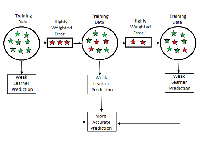
Gradient Boosting in the machine learning. A photo by Author

Hello Everyone, In this article, we will discuss the ensemble boosting techniques that is gradient boosting. In an earlier article on ensemble, we discussed random forest that is a bagging technique. In boosting the weak learners’ predict on the training set and the error/residual left with their weights are forwarded highly weighted ones’ to the next weak learner.

We saw Gini, Entropy in bagging techniques but in the case of boosting we will deal with loss functions because highly weighted loss goes to the next base learner. So, the last base learner gives the best prediction based on less error, and then combined prediction is well suited for the model.

n boosting methods, we try to reduce the bias while the prediction is based sequential-wise.

Gradient boosting is a sequential model in which the error is reduced with the help of gradient descent and makes a model in a form of a base model.

The advantages of Gradient boosting as shown below:

It reduces the bias.
Handle missing values in the data set.
Flexible to handle hyperparameter tuning.
Handling errors as a part of loss function via gradient descent.
Boosting classification handle both binary and multi-class problems.

Some of the loss function used in classification and regression with the help of loss parameter as shown below:

For Regression:

LAD – least absolute deviation: It deals with the median of the target value in the regression.
LS – least-square: It deals with the mean of the target value in the regression.
Huber: It is a combination of both LAD and LS for computation. To control the sensitivity we use the alpha parameter in the case of outliers.

For Classification:

Binomial deviance: This loss function works on binary classification with a basis on log odd ratio.
Multinomial deviance: The likelihood in loss function used in multi-class classification. When the class become increases then the regression trees as per given in n_class parameter become inefficient to make probabilities.
Exponential loss: It is only used in binary classification. This is also used in Adaboost classification.

Important points to remember:

The model is trained on sub-sample in stochastic gradient boosting that combines gradient boosting with bagging averaging (bootstrap).
The learning rate is via shrinkage is used for the regularization strategy. The shrinkage is used to make the number of iterations less.
The classification in gradient boosting is similar to regression so the value that comes from the tree is not class-wise rather it comes as a continuous value. So, for binary classification, we modeled with sigmoid function and for multi-class we use softmax.
The default metric used in classification with criterion parameter is ‘friedman_mse’. It measures the quality of the split. This default metric is very useful to give a better approximation than MSE and MAE.

An example of Titanic Dataset with python.

Import the libraries

import pandas as pd
from sklearn.preprocessing import MinMaxScaler
from sklearn.model_selection import train_test_split
from sklearn.metrics import classification_report, confusion_matrix
from sklearn.ensemble import GradientBoostingClassifier

MinMaxScaler is for scaling the values and here we will use the boosting classifier.

The data set consist of two files. Train and test CSV files. To read these files we used pandas.

train_data = pd.read_csv("train.csv")
test_data = pd.read_csv("test.csv")

A view of train data set.

Train set. A photo by Author

Now we will do some pre-processing and select the output column that survived in the y_train variable and removed it from the features data set. Here, the inplace is true because we want the changes in the original data set also.

y_train = train_data["Survived"]
train_data.drop(labels="Survived", axis=1, inplace=True)

Add the test set to the train set.

full_data = train_data.append(test_data)

As a part of feature engineering we can drop some columns that are not so much useful.

drop_columns = ["Name", "Age", "SibSp", "Ticket", "Cabin", "Parch", "Embarked"]
full_data.drop(labels=drop_columns, axis=1, inplace=True)

Now we will do encoding on the categorical column. The pandas provide get_dummies method to label the categorical values to numerical values.

full_data = pd.get_dummies(full_data, columns=["Sex"])
full_data.fillna(value=0.0, inplace=True)

Now split in train and test after pre-processing.

X_train = full_data.values[0:891]
X_test = full_data.values[891:]

Before modeling, scaling is a important step to standardize the values and divide the data in training and testing set..

scaler = MinMaxScaler()
X_train = scaler.fit_transform(X_train)
X_test = scaler.transform(X_test)state = 12  
test_size = 0.30  

X_train, X_val, y_train, y_val = train_test_split(X_train, y_train,  
    test_size=test_size, random_state=state)

Now we will try to fit the model and evaluate the accuracy with different learning rate.

lrate_list = [0.05, 0.075, 0.5, 0.75, 1]

for learning_rate in lrate_list:
    gb_clf = GradientBoostingClassifier(n_estimators=20
    , learning_rate=learning_rate, max_features=2, max_depth=2,
     random_state=0)    gb_clf.fit(X_train, y_train)

    print("Learning rate: ", learning_rate)
    print("Accuracy score (training):
               {0:.3f}".format(gb_clf.score(X_train, y_train)))
    print("Accuracy score (validation):
               {0:.3f}".format(gb_clf.score(X_val, y_val)))

Performance with different learning rate. A photo by Author

From the above performance we saw that the validation score is good with “0.5” learning rate. Now, we will predict out model with this value.

gb_clf2 = GradientBoostingClassifier(n_estimators=20,
     learning_rate=0.5, max_features=2, max_depth=2, random_state=0)gb_clf2.fit(X_train, y_train)
predictions = gb_clf2.predict(X_val)

print("Confusion Matrix:")
print(confusion_matrix(y_val, predictions))

print("Classification Report")
print(classification_report(y_val, predictions))#output:Confusion Matrix:
[[142  19]
 [ 42  65]]
Classification Report
              precision    recall  f1-score   support

           0       0.77      0.88      0.82       161
           1       0.77      0.61      0.68       107

    accuracy                           0.77       268
   macro avg       0.77      0.74      0.75       268
weighted avg       0.77      0.77      0.77       268

Conclusion:

Gradient boosting gives very good result in both classification and regression.

I hope you like the article. Reach me on my LinkedIn and twitter.