Machine Learning For Beginners: Classifying Iris Species

Original Source Here

A First Application: Classifying iris species

We will go through a simple machine learning application and create our first model. In the process, we will introduce some core concepts and nomenclature for machine learning.

Meet the data

The Iris flower data set or Fisher’s Iris data set is a multivariate data set. The data set consists of 50 samples from each of three species of Iris (Iris setosa, Iris virginica and Iris versicolor). Four features were measured from each sample: the length and the width of the sepals and petals, in centimetres. Based on the combination of these four features, Fisher developed a linear discriminant model to distinguish the species from each other.

Preview of Data
There are 150 observations with 4 features each (sepal length, sepal width, petal length, petal width).
There are 50 observations of each species (setosa, versicolor, virginica).

It is included in scikit-learn in the dataset module. We can load it by calling the load_iris function:

from sklearn.datasets import load_iris
iris = load_iris()

The iris object that is returned by load_iris is a Bunch object, which is very similar to a dictionary. It contains keys and values:

iris.keys()Out[3]: dict_keys(['DESCR', 'data', 'target_names', 'feature_names', 'target'])

The value to the key DESCR is a short description of the dataset. We show the beginning of the description here.

print(iris['DESCR'][:193] + "\n...")Out[4]:
.. _iris_dataset:

Iris plants dataset
--------------------

**Data Set Characteristics:**

    :Number of Instances: 150 (50 in each of three classes)
    :Number of Attributes: 4 numeric, pre
...

The value with key target_names is an array of strings, containing the species of flower that we want to predict:

iris['target_names']Out[5]:
array(['setosa', 'versicolor', 'virginica'], dtype='<U10')

The feature_names are a list of strings, giving the description of each feature:

iris['feature_names']Out[6]: 
['sepal length (cm)',
 'sepal width (cm)',
 'petal length (cm)',
 'petal width (cm)']

The data itself is contained in the target and data fields. The data contains the
numeric measurements of sepal length, sepal width, petal length, and petal width in a numpy array:

type(iris['data'])Out[7]:
numpy.ndarray

The rows in the data array correspond to flowers, while the columns represent the four measurements that were taken for each flower:

iris['data'].shapeOut[8]:
(150, 4)

We see that the data contains measurements for 150 different flowers.

Remember that the individual items are called samples in machine learning, and their properties are called features.

The shape of the data array is the number of samples times the number of features.

This is a convention in scikit-learn, and your data will always be assumed to be in this shape.
Here are the feature values for the first five samples:

iris['data'][:5]Out[9]:
array([[5.1, 3.5, 1.4, 0.2],
       [4.9, 3. , 1.4, 0.2],
       [4.7, 3.2, 1.3, 0.2],
       [4.6, 3.1, 1.5, 0.2],
       [5. , 3.6, 1.4, 0.2]])

The target array contains the species of each of the flowers that were measured, also as a numpy array:

type(iris[‘target’])Out[10]:
numpy.ndarray

The target is a one-dimensional array, with one entry per flower:

iris['target'].shapeOut[11]:
(150,)

The species are encoded as integers from 0 to 2:

iris['target']Out[12]:
array([0, 0, 0, 0, 0, 0, 0, 0, 0, 0, 0, 0, 0, 0, 0, 0, 0, 0, 0, 0, 0, 0, 0, 0, 0, 0, 0, 0, 0, 0, 0, 0, 0, 0, 0, 0, 0, 0, 0, 0, 0, 0, 0, 0, 0, 0, 0, 0, 0, 0, 1, 1, 1, 1, 1, 1, 1, 1, 1, 1, 1, 1, 1, 1, 1, 1, 1, 1, 1, 1, 1, 1, 1, 1, 1, 1, 1, 1, 1, 1, 1, 1, 1, 1, 1, 1, 1, 1, 1, 1, 1, 1, 1, 1, 1, 1, 1, 1, 1, 1, 2, 2, 2, 2, 2, 2, 2, 2, 2, 2, 2, 2, 2, 2, 2, 2, 2, 2, 2, 2, 2, 2, 2, 2, 2, 2, 2, 2, 2, 2, 2, 2, 2, 2, 2, 2, 2, 2, 2, 2, 2, 2, 2, 2, 2, 2, 2, 2, 2, 2])

The meaning of the numbers are given by the iris[‘target_names’] array: 0 means Setosa, 1 means Versicolor and 2 means Virginica.

Measuring Success: Training and testing data

We want to build a machine learning model from this data that can predict the species of iris for a new set of measurements.

Before we can apply our model to new measurements, we need to know whether our model actually works, that is whether we should trust its predictions.

Unfortunately, we can not use the data we use to build the model to evaluate it. This is because our model can always simply remember the whole training set, and will therefore always predict the correct label for any point in the training set. This “remembering” does not indicate to us whether our model will generalize well, in other words, whether it will also perform well on new data. So before we apply our model to new measurements, we will want to know whether we can trust its predictions.

To assess the models’ performance, we show the model new data (that it hasn’t seen before) for which we have labels. This is usually done by splitting the labelled data we have collected (here our 150 flower measurements) into two parts.

The part of the data is used to build our machine learning model and is called the training data or training set. The rest of the data will be used to access how well the model works and is called test data, test set or hold-out set.

Scikit-learn contains a function that shuffles the dataset and splits it for you, the train_test_split function.

This function extracts 75% of the rows in the data as the training set, together with the corresponding labels for this data. The remaining 25% of the data, together with the remaining labels are declared as the test set.

How much data you want to put into the training and the test set respectively is somewhat arbitrary, but using a test-set containing 25% of the data is a good rule of thumb.

In sci-kit-learn, data is usually denoted with a capital X, while labels are denoted by a lower-case y .

Let’s call train_test_split on our data and assign the outputs using this nomenclature:

from sklearn.model_selection import train_test_split
X_train, X_test, y_train, y_test = train_test_split(iris['data'], iris['target'],random_state=0)

The train_test_split function shuffles the dataset using a pseudo random number generator before making the split. If we would take the last 25% of the data as a test set, all the data point would have the label 2 , as the data points are sorted by the label (see the output for iris[‘target’] above). Using a tests set containing only one of the three classes would not tell us much about how well we generalize, so we shuffle our data, to make sure the test data contains data from all classes.

To make sure that we will get the same output if we run the same function several times, we provide the pseudo random number generator with a fixed seed using the random_state parameter. This will make the outcome deterministic, so this line will always have the same outcome.

The output of the train_test_split function are X_train , X_test , y_train and
y_test , which are all numpy arrays. X_train contains 75% of the rows of the dataset, and X_test contains the remaining 25%:

X_train.shapeOut[13]: (112, 4)X_test.shapeOut[14]:(38, 4)

First things first: Look at your data

Before building a machine learning model, it is often a good idea to inspect the data, to see if the task is easily solvable without machine learning, or if the desired information might not be contained in the data.

Additionally, inspecting your data is a good way to find abnormalities and peculiarities. Maybe some of your irises were measured using inches and not centimeters, for example. In the real world, inconsistencies in the data and unexpected measurements are very common.

One of the best ways to inspect data is to visualize it. One way to do this is by using a scatter plot. A scatter plot of the data puts one feature along the x-axis, one feature along the y-axis, and draws a dot for each data point.

Unfortunately, computer screens have only two dimensions, which allows us to only plot two (or maybe three) features at a time. It is difficult to plot datasets with more than three features this way.

One way around this problem is to do a pair plot, which looks at all pairs of two features. If you have a small number of features, such as the four we have here, this is quite reasonable. You should keep in mind that a pair plot does not show the interaction of all of features at once, so some interesting aspects of the data may not be revealed when visualizing it this way.

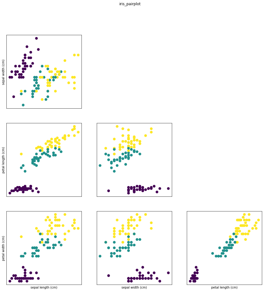
Here is a pair plot of the features in the training set. The data points are colored according to the species the iris belongs to:

import matplotlib.pyplot as pltfig, ax = plt.subplots(3, 3, figsize=(15, 15))
for i in range(3):
    for j in range(3):
        ax[i, j].scatter(X_train[:, j], X_train[:, i + 1],c=y_train, s=60)
        ax[i, j].set_xticks(())
        ax[i, j].set_yticks(())
        if i == 2:
            ax[i, j].set_xlabel(iris['feature_names'][j])
        if j == 0:
            ax[i, j].set_ylabel(iris['feature_names'][i + 1])
        if j > i:
            ax[i, j].set_visible(False)        plt.suptitle("iris_pairplot")

From the plots, we can see that the three classes seem to be relatively well separated using the sepal and petal measurements. This means that a machine learning model will likely be able to learn to separate them.

Next, we will look into k nearest neighbors..!!

AI/ML

Trending AI/ML Article Identified & Digested via Granola by Ramsey Elbasheer; a Machine-Driven RSS Bot

via WordPress https://ramseyelbasheer.wordpress.com/2021/01/31/machine-learning-for-beginners-classifying-iris-species/