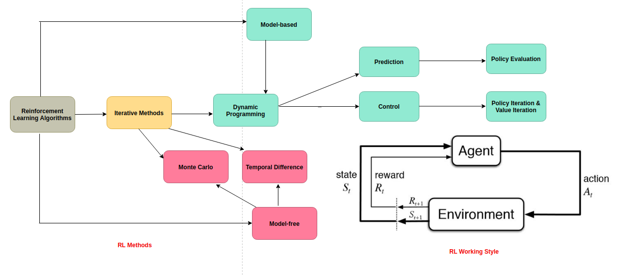
Reinforcement Learning & Deep RL
Original Source Here
Markov Decision Process (MDPs) plays a vital role in nondeterministic search problems ,it deals with multiple successor states in an efficient way and it is mainly considered as offline planning and agents has full knowledge of the transitions and reward ( or environment). MDP provides the formalism in which RL problems are usually posed.
A Markov Decision Process is defined by several properties. A Markov Decision Process is a tuple and it is defined as
Where:
The future is independent of the past given the present. A state is said to be Markov if and only if:
The state captures all relevant information from the history. Once the state is known, the history may be thrown away i.e., The state is a sufficient statistic of the future.
MDP can be modeled as state action reward sequence
The Reward Function is defined as ,
Return Function is the total discounted reward from time-step t and is defined as
The Value function V(s) describes the long-term value of state s. Value Functions has different variants and described shortly.
The state value function V(s) is the expected return starting from state s
Value function can be decomposed into Immediate reward and discounted value of successor state.
Immediate Reward and Discounted value of Successor state
It is a necessary condition for optimality associated with the mathematical optimization method known as Dynamic Programming.
DP simplifies a complicated problem by decomposing into simple sub-problems in a recursive manner.
Optimal Substructure: A complex problem can be solved optimally by decomposing into sub-problems and using a recursive concept for finding optimal solutions to the sub-problems, then it is Optimal Substructure.
Sub-problems can be nested recursively inside larger problems, so that DP methods are applicable, then there is a relation between the value of the larger problem and the values of the sub-problems. In the optimization literature this relationship is called the ”Bellman Equation”.
The Bellman equation can be expressed concisely using matrices,
Value Function has variants which require policy. They are State-Value Function and Action-Value Function, which will discuss after policy definition.
A Policy is a distribution over actions given states,
A policy fully defines the behavior of an agent. MDP policies depend on the current state (not the history) i.e., Policies are stationary (time-independent)
The state transition and reward function are incorporated with policies and is defined as follows
The State-Value function is the expected return starts from state s, and then following policy
The Action-Value function is the expected return starts from state s, taking action a and then following policy
The state-value and action-value function can be decomposed into immediate reward plus discounted value of successor state
Bellman expectation equation for state-value function can be expressed in matrix form is as follows
Optimality for state-value, action-value and policy.
Optimal state-value function
Optimal action-value function
The optimal value function specifies the best possible performance and once known it is marked as solved in MDP.
Optimal Policy
Defining a partial ordering over policies is as follows
An optimal policy can be found by maximizing over optimal value action
The optimal value functions are recursively related by the Bellman optimality equations:
RL derives some of the concepts of MDP for algorithms as already been stated that it provides the formalism in which RL problems are usually posed.
Let us consider an example which has 3 states of a car and evaluate the required functions from these.
As you have seen in this example rewards specified with (+/-) sign , actions (slow, fast) and transitions without sign. Based on this graph we need to calculate Value functions and Policies.
Let us construct Transition function and Reward function table and use in value and policy iterations.
Before we start to evaluate or examine we need Value Iteration, Policy Extraction and Policy Iteration.
Value iteration used for computing the optimal values of states, by iterative updates until convergence.
Value Iteration is a Dynamic Programming algorithm that uses iteratively longer time limit to compute time-limited values until convergence i.e., V values are the same for each state at time ‘k’ and ‘k+1’. By the definition it would be
It operates is as follows
Computation of Value Iteration:
Step 1:We begin set initial state to zero i.e.,
Step 2: In our first round of updates, we can compute first state (Cool State)
AI/ML
Trending AI/ML Article Identified & Digested via Granola by Ramsey Elbasheer; a Machine-Driven RSS Bot
via WordPress https://ramseyelbasheer.wordpress.com/2020/12/31/reinforcement-learning-deep-rl/