Learning Neural Networks: Intro to CNN using Keras to classify Rock, Paper, Scissors Images
Original Source Here
Learning Neural Networks: Intro to CNN using Keras to classify Rock, Paper, Scissors Images
For the longest time, Neural Networks was one of the topics I was eager to learn the most not only because of their application in many incredible tasks such as Image Recognition and Natural Language Processing, but because I could never wrap my head around the fact that many of the advancements in the field came from research in the way our own brain works. To think that something as complex as the brain’s architecture is somehow replicable and even more so, that we’ve managed to make it work is mind blowing. One of my early encounters with Machine Learning was reading The Master Algorithm by Pedro Domingos. In his book, Domingos describes the quest for the ultimate learning machine and the implications of such a learner, and along the way, he explains the progress there has been in the field of AI. Domingos explained the different tribes in Machine learning, and one really surprised me:
“Connectionists reverse engineer the brain and are inspired by neuroscience and physics.”
How can we teach a computer explicitly how to perform tasks the way the brain does? Another quote made me cringe even more:
“The number of connections in your brain is over a million times the number of letters in your genome, so it’s not physically possible for the genome to specify in detail how the brain is wired.”
How could we code up something that not even Nature explicitly codes?
Therein lies the answer. I didn’t understand the power of learning.
As with the other 3 phases in the Data Science Bootcamp I’m enrolled in, the last phase of my 10 month bootcamp culminates with a project. The content for this last phase included topics such as Dimensionality Reduction, Natural Language Processing, Perceptrons and other building blocks of Deep Learning. So before getting my boots dirty and delving into my actual Phase Project, which consisted in classifying X ray pictures of Patients with Pneumonia and Healthy patients, I decided to try a mini project and explore the TensorFlow Datasets (TFDS), which include dozens of datasets for you to explore.
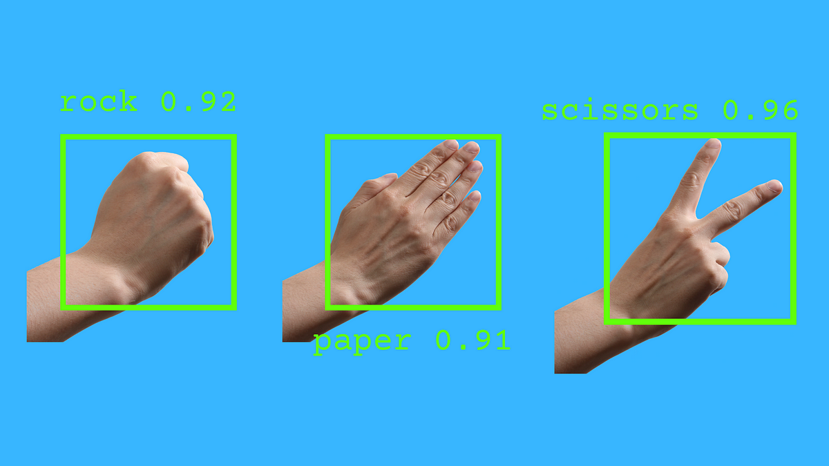
We’ll use a very particular dataset created by digital artist Laurence Moroney, who in his own words “wanted to see if [he] could use Photoreal CGI to train a neural network that could then recognize and classify real images with the same subject matter.” This adds another layer of flavor to this project because we’re not dealing with the typical datasets that beginners start out with, such as the MNIST handwritten digit database.
Let’s take a look at some examples of the dataset we’ll be working with:
fig = tfds.show_examples(info, train)
As you can see, the hands are computer generated and some are even on the funky side. Let’s get started
Training a NN
Before we get to CNN, let’s train a basic Neural Network with a couple of hidden layers. This Neural Network basically fully connects all the pixels in the image to the neurons and adjusts them accordingly:
model = keras.Sequential([
    keras.layers.Flatten(),
    keras.layers.Dense(512, activation='relu'),
    keras.layers.Dense(256, activation='relu'),
    keras.layers.Dense(3, activation='softmax')
])model.compile(optimizer='adam',
             loss=keras.losses.SparseCategoricalCrossentropy(),
              metrics=['accuracy']) model.fit(train_images, train_labels, epochs=5, batch_size=32)
We can see that with each epoch, the network gets better and better at classifying the image. Pretty neat right? Let’s see how well it does with our test set, which includes images that our network has never seen before:
model.evaluate(test_images, test_labels)
The accuracy for the test data dropped from 83% to 56%. So the model is practically useless when classifying images it’s never seen before. So what is going on here?
In general, Deep Neural Network with fully connected layers “work fine for small images(eg. MNIST), but it breaks down for larger images because of the huge number of parameters it requires.”(Géron) They are also prone to overfitting which as you probably know is one of the most common problems in deep learning models.
Enter Convolutional Neural Networks
We will attempt to solve this problem by using convolutional layers, the bedrock of CNN. The origins of CNN can be traced to early research on the way cats and monkeys see. Long story short, neurons in the visual cortex react to a limited local receptive field, so a single neuron for example, reacts to a certain part of the whole image you see.
I know this sounds very confusing, but the important part is that a single neuron is not connected to every single visual input. In the context of image recognition, a single neuron in the first layer wouldn’t be connected to all of the pixels in an image. This allows our layers to recognize generalizable features and make a more concrete decision when classifying the object. In the network we just coded, we were focusing too much attention in the single pixels.
Let’s brew a simple CNN:
model = keras.Sequential([
    keras.layers.Conv2D(64, 3, activation='relu', input_shape=(300,300,1)),
    keras.layers.Conv2D(64, 3, activation='relu'),
    keras.layers.Flatten(),
    keras.layers.Dense(3, activation='softmax')
])model.compile(optimizer='adam',
             loss=keras.losses.SparseCategoricalCrossentropy(),
              metrics=['accuracy'])model.fit(train_images, train_labels, epochs=5, batch_size=32)
100% Accuracy?! That sounds insane, but is our model really that good?
First, let’s go through the lines of codes to understand the components and parameters that make up our model. As you can see from the first block of code, our model contains 4 layers. The first 2 layers are our convolutional layers, which transform our images. Each filter produces what we call a feature map that is then fed to subsequent filters in other layers. For each layer, we specify parameters such as how many filters the layer contain, the kernel size, stride and activation function. I won’t get into what each of these mean but this video by Brandon Rohrer does a fantastic job of explaining them. Next, we flatten our maps into a single, one dimensional vector with the hope that by this point, our convolutional layers have “identified” generalizable features, like shapes and edges. Then this one dimensional vector is fed to the last layer, which acts as the actual classifier using softmax as the activation function. In ultra simplified terms, this last layer hopefully looks at our 1D vector and classifies the image based on the features it has identified (eg. This image contains tires, a windshield and it looks like its on a road, it’s probably a car).
Something worth noting is how much longer this model took to train. In total, it took more than 43 minutes to run through the training data and adjust the layers. One way of making this more efficient is by running this Jupyter Notebook script with the GPU, which makes this training process a lot faster.
So well, was the wait worth it? let’s take a look at how well it does with our test split:
model.evaluate(test_images, test_labels)
Oof, not so good now. One thing we haven’t mentioned at all is how little data is contained in our training sets. When dealing with a shortage of data, there are a couple of options. To deal with this problem I’ll use a regularization technique commonly used when networks overfit or when there is very little data. We’ll come back to this later on.
An Improved Convolutional Network
So what can we do to fix this? Another important building block in convolutional networks is the Pooling Layer. Pooling layers solve a couple of problems like computational complexity, memory usage and add invariance to small translations in the picture. In other words, Max pooling for example allows our model to identify a tire even if it’s a couple of pixels to the left of where the model is used to seeing a tire. Again, this is a very simplified explanation, but for now let’s try adding a couple of this pooling layers to our model.
model = keras.Sequential([
 keras.layers.AveragePooling2D(6,3, input_shape=(300,300,1))
    keras.layers.Conv2D(64, 3, activation='relu', input_shape=(300,300,1)),
    keras.layers.Conv2D(64, 3, activation='relu'),
keras.layers.MaxPool(2,2),
    keras.layers.Flatten(),
keras.layers.Dense(128, activation='relu')
    keras.layers.Dense(3, activation='softmax')
])
Let’s break down our upgrades to the model, which you can find as the bold lines in the code block above:
- We start out with an average pooling layer, which reduces our image size to 1/3 of its initial size.
- Another pooling layer is added after our convolutional layers, this time a max pooling layer, probably the most used type of pooling type. You can expect a better performance during training when adding pooling layers because it reduces significantly the operations performed (in the process we lose information because we’re reducing the size of the images)
- Finally, I added a hidden layer before our output layer, which will help our model with the classification task. This hidden layer uses ReLU as its activation function.
Let’s run this model:
model.evaluate(test_images, test_labels)
Okay, a little bit better than our previous model, but still our classifier is not that good at doing its task. One thing I haven’t mentioned is that we’ve been looking at the accuracy as our only success metric when determining whether our model is doing a good job at classifying these images. We’ll come back to this topic in a bit. Let’s try to improve our model one last time:
model = keras.Sequential([
    keras.layers.AveragePooling2D(6,3, input_shape=(300,300,1)),
    keras.layers.Conv2D(64, 3, activation='relu', input_shape=(300,300,1)),
    keras.layers.Conv2D(128, 3, activation='relu'),
    keras.layers.MaxPool2D(2,2),
 keras.layers.Conv2D(128, 3, activation='relu', input_shape=(300,300,1)),
    keras.layers.Conv2D(256, 3, activation='relu'),
    keras.layers.MaxPool2D(2,2),
 keras.layers.Dropout(0.5),
    keras.layers.Flatten(),
    keras.layers.Dense(128, activation='relu'),
    keras.layers.Dense(3, activation='softmax')
])
This time, we added an extra 2 layers of convolution, and a MaxPool layer. We can think of these 3 layers as a block, and we can keep stacking blocks of convolution and pooling on top of each other. Notice how the number of filters in the convolution layers grows as we climb up the CNN (64, 128 and then 256). As Aurélien Géron puts it, “it make sense for it to grow, since the number of low-level features is often fairly low (eg. small circles, horizontal lines), but there are many different ways to combine them into higher level features.”
Finally, to combat the small number of training samples, we’ll use a dropout layer. Dropout layers are regularization tools that also help us combat overfitting. Let’s see how our new model does:
Now, let’s check the model’s confusion matrix, precision, recall and f1 score. In case you need to refresh on the topic of metrics, here’s a great article with the explanation of each metric. Let’s take a look at other metrics:
One thing to note is that the Confusion matrix is flipped in the x-axis. The confusion matrix shows us that from 124 images of rocks, our classifier identified 120 (!) correctly. This is outstanding, but remember that this is just one side of the coin. The classifier also mistakenly classified 72 pictures of scissors and paper as rocks. You can also see that it the classifier had a hard time classifying scissors: from 124 pictures of scissors it only classified 58 correctly as scissors. It seems like the model had an affinity to classify pictures of scissors as rocks.
Conclusions and Further steps
There is a ton of work to do if we wish to improve our classifier. Many models I found on Kaggle using the same datasets had similar accuracy results. Their confusion matrix obviously looked different, but the point is we got some pretty decent results by just building a basic CNN without tuning parameters. Something we could try if we wish to improve our metrics is using an automatic hyperparameter tuner that can check on many different combinations of them and finding the best one. Once we have the best one, we could save the models or extract these parameters to further improve our model.
We could also try using a pre-trained network and train over those layers. This is a very common practice when dealing with a shortage of training data and sometimes, we can even get lucky and find pre-trained models with similar dataset (imagine you’re training a model to identify types of bears and you find a pre-trained that was trained using images of wolverines)
Model tuning in NN apparently takes a lot of practice and intuition. Knowing what layers to add and which parameter values to pick is something that Data Scientist with more experience can do better. Even considering the possibility of automatically selecting the best hyperparameters as mentioned earlier, expertise and intuition still hold a huge importance when working with Deep Learning.
AI/ML
Trending AI/ML Article Identified & Digested via Granola by Ramsey Elbasheer; a Machine-Driven RSS Bot
via WordPress https://ramseyelbasheer.io/2021/05/31/learning-neural-networks-intro-to-cnn-using-keras-to-classify-rock-paper-scissors-images/