Cassava Leaf Disease Detection: Final Model and Predictions
Original Source Here
Cassava Leaf Disease Detection: Final Model and Predictions
By Brett Cotler and Alex Zimbalist
In this post, we show our final approach to classifying leaf disease from images as part of the Cassava Leaf Disease Detection Kaggle Competition. In our two previous posts on this topic, we laid much of the groundwork for what will be covered in the following paragraphs. Feel free to review our first (https://alex-zimbalist.medium.com/cassava-leaf-disease-classification-first-steps-9bc6a6478ec6) and second (https://alex-zimbalist.medium.com/cassava-leaf-disease-classification-part-ii-32476dc18c78) blog posts before reading further. To follow along with the code snippets presented throughout this post, you can access our Google Colab notebook here: https://colab.research.google.com/drive/19O85X_5AD_S5hifse_MpOyrCDjvKz_Ry?authuser=2#scrollTo=_YnFQNwjJwDY.
In our previous blog post, we fine-tuned an EfficientNetB6 model to make classification predictions. On a good run, this model could achieve 80% validation accuracy. We concluded the post by teasing future parameter and architecture tweaks that would hopefully improve upon this accuracy. We begin our discussion of these tweaks by revisiting our image data augmentation techniques.
Before any augmentation, the images look this:
We tried several different augmentations. Several of these are shown in the code snippet below.
data_augmentation = tf.keras.Sequential([layers.experimental.preprocessing.RandomFlip("horizontal_and_vertical"),layers.experimental.preprocessing.RandomRotation(0.2, fill_mode = 'constant'),layers.experimental.preprocessing.RandomContrast(factor=.5),layers.experimental.preprocessing.RandomTranslation(0.2, 0.2),layers.experimental.preprocessing.RandomZoom(0.3),layers.experimental.preprocessing.Rescaling(scale=1, offset=0.1)])
These augmentations are fairly self-explanatory, performing alterations such as flipping the image, rotating the image, adding contrast, shifting the image up, down, or side to side, zooming in and out, etc. When we perform all the augmentations at once, the augmented images look like this:
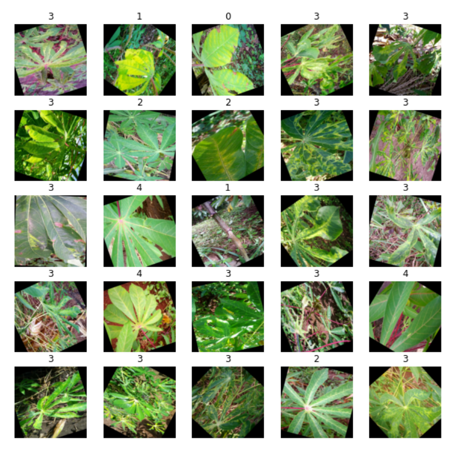
From playing around with numerous combinations of these augmentations, we actually found that less is more. Providing too much augmentation significantly hindered the model’s ability to produce high accuracies. Some augmentation is important so that the model knows how to make good predictions for images taken on different cameras, at different angles, with different levels of blurriness, saturation, contrast, etc. Further, augmentation tends to mitigate overfitting. With that being said, over-augmenting images to the point that they no longer resemble the types of images that we might want to classify provides little benefit and diminishes the model’s ability to identify the key features of each class. We ultimately settled on just a flip and a rotation:
data_augmentation = tf.keras.Sequential([layers.experimental.preprocessing.RandomFlip("horizontal_and_vertical"),layers.experimental.preprocessing.RandomRotation(0.2, fill_mode = 'constant')])
The augmented images look like this:
We tried producing classification models by fine-tuning 3 different pre-trained convolutional neural networks: VGG16, ResNet50, and EfficientNetB0. We should note here that we originally chose to use ResNet101 and EFficientNetB6, but these models simply had too many trainable parameters for our Google Colab notebook to handle. In order to use ResNet50 and EfficientNetB0, we had to resize the images to be 224 pixels by 224 pixels, rather than 512 by 512. This resizing is done in the decode_image function, as shown below:
def decode_image(image):
    image = tf.image.decode_jpeg(image, channels=3)
    image = tf.reshape(image, [*IMAGE_SIZE, 3])
    image = tf.cast(image, tf.float32)
    image = tf.image.resize(image, [224, 224])
    return image
For the sake of brevity, we will show only the code for our ResNet model. However, the code for our EfficientNet and VGG16 models are nearly identical (just with “res” with “efficient” or “vgg” in a couple of places!).
The basic model architecture we settled on looks like this:
shape=(224, 224, 3)base_model = ResNet50(input_shape=shape, include_top=False, weights="imagenet")base_model.trainable = Falseinputs = Input(shape=shape)
x = data_augmentation(inputs)
x = tf.keras.applications.resnet.preprocess_input(x)
x = base_model(x, training=False)
x = GlobalAveragePooling2D()(x)predictions = Dense(5, activation = 'softmax')(x)model2 = Model(inputs, predictions)
There are two important things to note here that changed since our last blog post. First, we note that Flatten() has been replaced with GlobalAveragePooling2D(). There are two reasons for this. First, global average pooling gave us better results experimentally. Second, flattening treats all the pixels in an image as being independent of one another. Of course, this is not the case, as pixels along one column of pixels in an image are often highly correlated (for instance, a vertical strip through an image might entirely consist of background, in which case every pixel would be nearly identical). Global average pooling makes no such assumption of independence. The second notable change from our previous attempts is that we decided not to add any dense layers on top of the pre-trained model. Once again, part of our reason for making this decision was experimentation and trial and error. Simply put, no matter how many dense layers we added and no matter how many neurons we put in each dense layer, we were hard-pressed to find a combination that improved model performance. Additionally, after initially training the model, we unfreeze the base model and then re-compile and re-fit. This step allows the model to learn better convolutional filters that are specific to cassava leaf disease classification. By unfreezing the base model and re-compiling and re-fitting, adding dense layers on top of the base model is entirely unnecessary.
In order to optimize performance, we introduce three callbacks:
early_stopping = EarlyStopping(monitor = 'val_loss', mode = 'min',
    patience = 5, min_delta = 1e-3)reduce_lr = ReduceLROnPlateau(monitor='val_loss', factor=0.2,
    patience=3, min_lr=1e-5)model_checkpoint = ModelCheckpoint(filepath='/checkpoint',
    save_weights_only=True, monitor='val_accuracy', mode='max',
    save_best_only=True)
Early stopping tells our model to stop training if the validation loss has not “beaten” the best previous validation loss by more than 0.001 for 5 consecutive epochs. This serves two purposes. First, early stopping can prevent overfitting, terminating the training process when validation loss stops improving even if the training loss is continuing to decrease. Second, the callback saves us training time. We set the number of epochs to 100, but the model never comes close to training for this long due to early stopping.
The second callback we introduce is ReduceLROnPlateau. This callback, like early stopping, monitors validation loss. Based on the parameters we chose for the callback, if the validation loss fails to beat the previously best validation loss for 3 consecutive epochs, the learning rate is multiplied by 0.2. This allows us to start with a very large initial learning rate (we chose 0.01) that decreases to the minimum learning rate, which we defined as 1e-5. Like early stopping, this callback speeds up training by allowing us to start with a very large learning rate. Additionally, the callback helps prevent the optimizer from “settling into” a bad local minimum rather than finding the true global minimum.
Finally, we have a callback called ModelCheckpoint, which keeps track of the best validation result during the training process. It is often the case that the last epoch before training terminates does not produce the best results; in this case, we want to choose for our model the weights from the epoch that produced the best results. ModelCheckpoint does exactly this.
Next, we compile and fit the model.
model2.compile(optimizer = Yogi(learning_rate=base_learning_rate),
    loss = 'sparse_categorical_crossentropy',
    metrics = ['accuracy'])history2 = model2.fit(train_dataset,
    validation_data = validation_dataset,
    callbacks = [early_stopping, reduce_lr, model_checkpoint],
    epochs = 100,
    verbose = 1)model2.save('./model2_fully_frozen_tf',save_format='tf')
There are two things to note in the code snippet above. First, we chose to use the optimizer Yogi. This choice is admittedly somewhat arbitrary, but after playing around with both Adam and Yogi, we determined that the Yogi optimizer performs at least as well, if not better. Second, we save the results of the model in the last line of the code above. While this is not strictly necessary, it is a good tool to use when working in Google Colab — if the notebook times out due to inactivity, trained model weights will be lost unless they are saved, as shown.
The results of the model so far described are shown here, beginning from epoch 20.
As we can see, the training process is terminated by early stopping after 32 epochs. We achieved a validation accuracy of just under 75% at epoch 27, and due to the model checkpoint callback, these are the model weights that we retain. As hinted at previously, the next step is to unfreeze the base model and re-compile and re-fit, as this allows the model to learn convolutional filters that are specific to the images we are trying to classify.
base_model.trainable = Truebase_learning_rate = 1e-4reduce_lr_2 = ReduceLROnPlateau(monitor='val_loss', factor=0.2, patience=3, min_lr=1e-8)model2.load_weights('/checkpoint')model2.compile(optimizer = Yogi(learning_rate=base_learning_rate),
    loss = 'sparse_categorical_crossentropy',
    metrics = ['accuracy'])history2 = model2.fit(train_dataset,
    validation_data = validation_dataset,
    callbacks = [early_stopping, reduce_lr_2, model_checkpoint],
    epochs = 100,
    verbose = 1)model2.save('./model2_unfrozen_tf',save_format='tf')
Before unfreezing the base model, we had already attained approximately 75% validation accuracy — not amazing, but still pretty solid. The code above is really just trying to make slight tweaks to bump up this accuracy. Therefore, we set the initial learning rate to be pretty small (1e-4), and allow it to get as low as 1e-8 as the learning rate is reduced as validation loss plateaus. Indeed, this approach yields significantly improved validation accuracy.
At epoch 14, validation accuracy reached just under 85%. This is a vast improvement over what our prior models had been able to produce! While we will not show this code again for the EfficientNet or VGG16 models, the results are displayed below.
EfficientNet performs nearly as well as ResNet, achieving just under 84% validation accuracy compared to just under 85% validation accuracy for ResNet. VGG16 actually performs slightly better than both ResNet and EfficientNet, reaching maximum validation accuracy of just over 86%. We can visualize how all 3 models train with their respective base models unfrozen using the code below. Note that this code is adapted from code shown at https://machinelearningmastery.com/display-deep-learning-model-training-history-in-keras/. Once again, we show only the code for ResNet, since visualizing EfficientNet and VGG16’s training with the unfrozen base model uses nearly identical code.
# summarize history for accuracy from ResNet50 modelplt.plot(history.history['accuracy'])
plt.plot(history.history['val_accuracy'])
plt.title('model accuracy')
plt.ylabel('accuracy')
plt.xlabel('epoch')
plt.legend(['train', 'test'], loc='upper left')
plt.show()# summarize history for loss from ResNet50 modelplt.plot(history.history['loss'])
plt.plot(history.history['val_loss'])
plt.title('model loss')
plt.ylabel('loss')
plt.xlabel('epoch')
plt.legend(['train', 'test'], loc='upper left')
plt.show()
The results are shown below:
AI/ML
Trending AI/ML Article Identified & Digested via Granola by Ramsey Elbasheer; a Machine-Driven RSS Bot
via WordPress https://ramseyelbasheer.io/2021/03/21/cassava-leaf-disease-detection-final-model-and-predictions/


