A Closer Look Into The Math Behind Gradient Descent

Original Source Here

Table of Contents

1. Overview
2. Model
3. Forward Propagation
4. Backpropagation
5. Weight Updates
6. Conclusion

1. Overview

This article assumes familiarity with gradient descent.

For each node, we will first introduce a visual representation of the node and its inputs, then walkthrough the computations of transforming the inputs and applying the activation function.

The process of training a neural network is broken down into the following main steps:

Step 1: Forward propagation

• Training data is passed in a single direction through the network from input layer through the hidden layers and out through the output layer
• To train the network, we perform a forward pass by feeding the training data through the input layer, performing a series of multiplication and addition operations through the hidden layers, and outputting the final results in the output layers
• Input Layer → Hidden layers → Output layer

Step 2: Backpropagation

• After the output is computed through the forward pass, we measure how the prediction using pre-defined loss function. The loss function outputs an error value that tells us how well the network did. The error is then sent backward (backpropagated) through the network and the gradients are computed.
• Input Layer ← Hidden layers ← Output layer

Step 3: Update Weights

• The computed gradients tell us how much each weight affects the error and use the gradients to adjust the weights slightly (by parameter alpha rate) towards the target values
• w_i -= α * gradient_of_w_i

2. Model

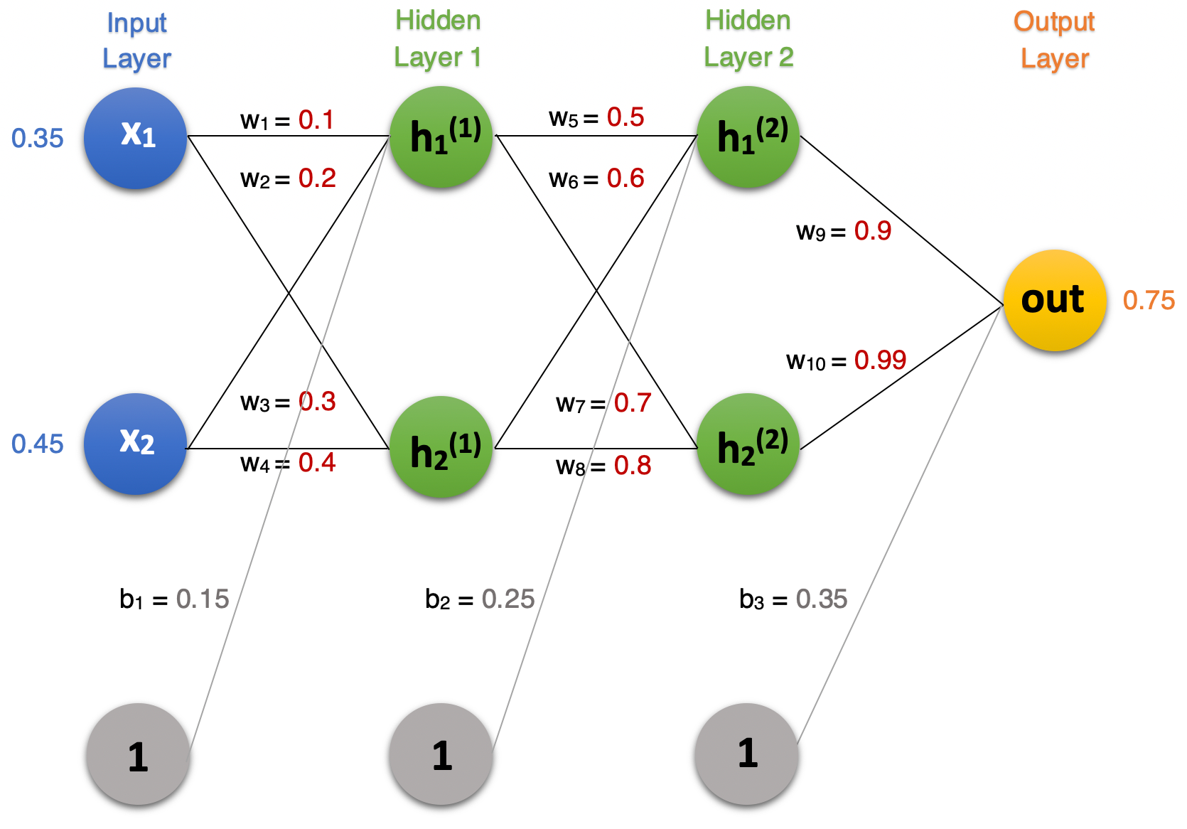
Here is our network architecture with 2 hidden layers and 1 output layer.

There are 2 input nodes, 2 hidden nodes in each of the hidden layers, and a single output node. The initial weights are given in red, the biases in gray, the input values in blue, and the target values in orange.

The image depicts a feed forward, fully-connected neural network.

• feedforward: means that the input moves forward through the network in a single direction in contrast to recurrent neural networks which have a loop that feeds outputs back into the network
• fully-connected: the nodes in each layer are connected to all nodes in previous and directly subsequent layer

3. Forward Propagation

In the forward pass, input data is transformed by weights and biases into z, then an activation is applied to the transformed input into a.

A single node

Step 1: Transform input data with weights and biases

Net of input

where l is the layer, n is the node number in the layer l, i index for the corresponding weight and input, and j is the size of the input vector

For each node, weights are combined with the inputs, then a bias term is added which allows the network to be shifted to better fit the data.

Step 2: Apply an activation function

An activation function is applied to the transformed input in the first part of the node in order to introduce non-linearly in the model. The activation function allows the model to build complex decision boundaries that can work with non-linearly separable data.

The activation function in this article is the Sigmoid Activation Function.

Final output of node

where l is the layer, n is the node number in the layer l.

Hidden Layer 1

Now that we have our net formulas and our activation function, we can compute the outputs for each individual node.

Hidden Node 1

Hidden Node 2

Hidden Layer 2

The inputs into the second hidden layer are the outputs of the previous H1 hidden layer that was computed above.

Hidden Node 1

Hidden Node 2

Output Layer

The inputs into the output node are the outputs of the second hidden layer nodes.

Output Node

The final predicted output of the network is 0.85049311458.

4. Backward Propagation

After the forward pass of the training sequence, we can now compute the accuracy of the network predictions by comparing the deviation of the outputs to the target values using a loss or error function.

In this article, we will use the squared loss function.

Squared Loss function

The constant 1/2 is included to simplify the differentiation of the loss function by cancelling out the exponent.

The loss is computed and backpropagated through all the layers using the chain rule. The computations in this section will start from the last layer, the output layer.

• Input Layer ← Hidden Layer 1 ← Hidden Layer 2 ← Output Layer

Derivatives

The derivatives needed to start the backward pass are the derivatives of the loss function and activation function. These will be chained together with subsequent derivatives as move back through the layers.

Squared Loss Derivative

Recall that the output of the network is a_out in the third layer or output layer.

Sigmoid Derivative

Assume that the input layer is constant for notation simplicity.

Recall:

Sigmoid Activation applied to net of weights and inputs + bias

Derivative of Sigmoid Function:

Hidden Layer 2 ← Output Layer

Now that we have the loss and sigmoid derivatives, we can compute the gradients of the weights connected directly to the output layer.

Recall:

The below visual is the final output node or the predictions of the network with its labeled inputs, weights, outputs, and target value. Refer to this image for values in the gradient computation.

Gradient of w_10

Derivative of loss w.r.t. w_10 using the Chain Rule

First term

Derivative of loss w.r.t. output (derived above)

Second term

Derivative of network prediction w.r.t transformed input

Third term

Derivative of z_out w.r.t. w_10

Combine Terms

Gradient of w_10

Gradient of w_9

Derivative of loss w.r.t. w_9 using the Chain Rule

Notice that the first two terms are the same as gradient of w_10. We can directly plug in the values from above.

Third term

Derivative of z_out w.r.t. w_9

Combine terms

Gradient of w_9

Hidden Layer 1← Hidden Layer 2

For the hidden weights in layer two preceding the output layer, the gradients depend on all the nodes in all subsequent layers. The error from all linked nodes gets backpropagated to the nodes in this layer. These nodes are affected by the error from the output node.

Gradient of w_5

The grayed out nodes and weights do not affect the gradient calculation of w_5.

Loss backward flow through colored nodes; ; bias terms omitted

Refer to the visual and notice how the loss flows from the output node (in orange) through w9 to hidden node 1 in layer 2, and through w5 to hidden node 1 in layer 1. The derivatives are chained together from the output node to w5.

Derivative of loss w.r.t w_5 using Chain Rule

First term

First term unrolled

When we unroll the first term, we see that the first two terms partial L w.r.t. a³_out and partial a³_out w.r.t. z³_out have already been computed in the gradient computations for w_10 and w_9. These previously computed values can be plugged in directly. Thus, we only need to compute the derivative of the last term partial z³_out w.r.t. a²_h1

Last term in unrolled first term

Plugging in the values in gives us

Derivative of first term in w5 computation

Second term

For the second and third terms, the derivatives are similar to calculating the derivatives for w_10 and w_9.

Derivative of a²_h1 w.r.t. z²_h1

Third term

Derivative of net of hidden node 1 in layer 2 w.r.t. w5

Putting it all together

Gradient of w5

Gradients of w_6, w_7, w_8

These gradients are computed the same as w_5 shown above, but the derivatives need to be taken w.r.t. to the weight we are attempting to compute. The gradients are given as follows

Gradients for the rest of the weights

Input Layer ← Hidden Layer 1

For the weights hidden weights in layer 1 preceding hidden layer 2, the gradients depend on all the nodes in all subsequent layers. Thus, the gradients of w_1, w_2, w_3, and w_4 are backpropagated from hidden layer 1, hidden layer 2, and the output layer.

Gradient of w_1

Visual of backward flow through colored nodes to w_1; bias terms omitted

To compute the gradient w_1, we need to once again use the chain rule.

Derivative of loss w.r.t w_5 using Chain Rule

Let’s look at each term individually.

Term 1

First term unrolled = Through H1 Node, Layer 2 + through H2 Node, Layer 2

After unrolling first term, we see that the first part is from Hidden Node 1 in layer 2 and the second part is from Hidden Node 2 in layer 2. Notice that both parts, the first four terms are have already been computed previously. The only term we need to compute is the last term or term 5 in each part.

• Last term through H1 Node in Layer 2

• Last term through H2 Node in Layer 2

We can now plug in all the values into the equation.

Combine

First term in gradient of w1

Term 2

Second term in gradient of w1

Term 3

Third term in gradient of w1

Putting it all together

Gradient of w1

Gradients of w_2, w_3, w_4

The gradients of w_2, w_3, and w_4 are computed similarly to w_1 by using the chain rule and backpropagating the loss through the weight. The gradients are given as follows:

5. Update Weights

Now that we have computed the gradients of all weights, we can update the weights so that the neural network predicts values that are closer to the target. The learning rate (α) is a value between 0 and 1.0 that represents how much of the gradient we will update the weight value towards. If the rate is too low, the neural network will learn very slowly. On the other hand, if the learning rate is set too high, the model may not converge. Thus, the learning rate is a parameter that can be optimized. In this article, we will use a learning rate of 0.5 for simplicity.

Update rule

Given initial weights

Given gradients

Weights after update

6. Conclusion

I hope this article was helpful in learning how input is transformed in the forward pass and how gradients are computed with the chain rule in the backward pass. Please let me know if there are any errors or if there are any improvements that can be made.

The same neural network is coded from scratch in NumPy here. The forward propagation and backward propagation code is unrolled so that it is easier to follow along with the current article.

If you’d like to see the same network coded from scratch in NumPy, the code is given here. The forward propagation and backward propagation code is unrolled so that it is easier to follow along with the current article.

AI/ML

Trending AI/ML Article Identified & Digested via Granola by Ramsey Elbasheer; a Machine-Driven RSS Bot

via WordPress https://ramseyelbasheer.wordpress.com/2021/01/23/a-closer-look-into-the-math-behind-gradient-descent/