Plant Disease Detection using Advanced Deep Learning and ReactJS
Original Source Here
First, we will design the Flask server to accommodate the pre-trained ResTS architecture. The server will incorporate a route to handle the input image coming from the application and will return a new image that comprises only the salient features along with the disease name and probability. Secondly, we will develop an uncomplicated React application where images can be uploaded and manifested. We will not go into the particulars regarding the ResTS architecture. Please follow the BELOW link to learn how this architecture operates to diagnose plant disease.
https://doi.org/10.1016/j.inpa.2021.06.001
1. Creating the server comprising our ResTS (Residual Teacher/Student) model
The architecture code is required to be put in the same file as the server. However, this can be changed but due to some errors, I decided to put the whole code of architecture in the same file and load the weights. Also, it is neat to have only one file to run instead of managing multiple files.
Source Code Access: You can find the links to the whole source code of this article and the ResTS architecture from the paper referenced above.
First, we will import all the necessary libraries into our Flask server file.
import os
from flask import Flask, request
import numpy as np
import matplotlib.pyplot as plt
import tensorflow as tf
import pandas as pd
import gevent.pywsgi
from flask_cors import CORS
from datetime import datetime
from tensorflow.python.keras.backend import set_session
from keras import backend as K
import tensorflow.compat.v1 as tf
import keras_preprocessing
from keras.applications.xception import preprocess_input as xception_preprocess_input
from keras_preprocessing import image
import json
from PIL import Image
from hashlib import sha256
###########################
from tensorflow.keras.layers import Input, Dense, Conv2D, Activation, MaxPool2D
from tensorflow.keras.layers import *
from tensorflow.keras.models import Model, Sequential
from tensorflow.keras.optimizers import Adam, SGD
import glob
import argparse
from keras import __version__
from keras.applications.xception import preprocess_input as xception_preprocess_input
from keras.preprocessing.image import ImageDataGenerator
from keras.optimizers import SGD
from keras import optimizers
from keras import callbacks
from keras.callbacks import ModelCheckpoint, LearningRateScheduler
from keras import backend as keras
from keras.regularizers import l2,l1
import pandas as pd
These will necessitate huge processing power. The next step is to define the ‘app’ variable with some other important variables and the session using the tf.session. tf.disable_v2_behavior() and tf.get_default_graph() was required while running the server to steer clear of any graph-related errors.
input_shape = (224,224,3)
nbr_of_classes=38
tf.disable_v2_behavior()
graph = tf.get_default_graph()app = Flask(__name__)
CORS(app)
sess = tf.Session()
set_session(sess)
Note: If the errors still occur during the starting phase of the server, there are high chances that it is due to the version error of TensorFlow. Try searching Stackoverflow in that case.
After defining the session, the architecture code will be implemented. ResTS uses standard Xception architecture as ResTeacher and ResStudent and the decoder is generated in the exact inverse manner of Xception architecture to reproduce the images. It is out of the scope of this article to discuss the ResTS architecture in-depth. To understand the below code properly, refer to the original paper.
#ResTS ARCHITECTURE#RESTEACHER
base_model1 = tf.keras.applications.Xception(include_top=False, weights='imagenet',input_shape = input_shape)
x1_0 = base_model1.output
x1_0 = Flatten(name='Flatten1')(x1_0)
dense1 = Dense(256, name='fc1',activation='relu')(x1_0)
x = classif_out_encoder1 = Dense(38, name='out1', activation = 'softmax')(dense1) # Latent Representation / Bottleneck#Get Xception's tensors for skip connection.
...#DECODER
dense2 = Dense(256, activation='relu')(x)x = Add(name='first_merge')([dense1, dense2])
x = Dense(7*7*2048)(x)
reshape1 = Reshape((7, 7, 2048))(x)#BLOCK 1
...#BLOCK 2
...#BLOCK 3-10
...#BLOCK 11
...#BLOCK 12
...#BLOCK 13
...#BLOCK 14
...x = Conv2D(2, 3, activation = 'relu', padding = 'same',)(x)
mask = x = Conv2D(3, 1, activation = 'sigmoid',name='Mask')(x)#RESSTUDENT
base_model2 = tf.keras.applications.Xception(include_top=False, weights='imagenet',input_shape = (224,224,3))
x2_0 = base_model2(mask)
x2_0 = Flatten(name='Flatten2')(x2_0)
x2_1 = Dense(256, name='fc2',activation='relu')(x2_0)
classif_out_encoder2  = Dense(nbr_of_classes, name='out2',activation='softmax')(x2_1)#Create ResTS Model and Load Pre-trained weights
ResTS = Model(base_model1.input, [classif_out_encoder1, classif_out_encoder2])
ResTS.load_weights('tf/RTS')
ResTS architecture is designed in a way such that it screens the noisy regions from the input image of the leaf with the help of an autoencoder. the mask layer is the output of the decoder that is taken for visualizing the important regions of the leaf image. classif_out_encoder1 that is the output of ResTeacher assists in classifying the disease category with the help of softmax function.
#For visualization impetuslayer_name ='Mask'
NewInput = ResTS.get_layer(layer_name).output
visualization = K.function([ResTS.input], [NewInput])
In the above code, visualization is a function that aids in getting the image comprising only the important features of the leaf image. Next, we will define some important functions for envisioning the features of an image received from the visualization function.
def reduce_channels_sequare(heatmap):
    channel1 = heatmap[:,:,0]
    channel2 = heatmap[:,:,1]
    channel3 = heatmap[:,:,2]
    new_heatmap = np.sqrt(((channel1-0.149)*(channel1-0.149))+((channel2-0.1529)*(channel2-0.1529))+((channel3-0.3412)*(channel3-0.3412)))
    return new_heatmap
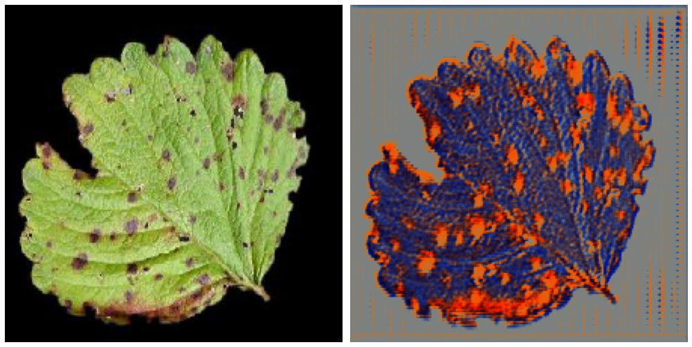
The reduce_channels_sequare function is required to convert the reconstructed RGB image into a one-channel image. It indirectly finds the distance between the dominant color in the reconstructed image (referred to as heatmap in this function).
def postprocess_vis(heatmap1,threshould = 0.9):
    heatmap = heatmap1.copy()
    heatmap = (heatmap - heatmap.min())/(heatmap.max() - heatmap.min())
    heatmap = reduce_channels_sequare(heatmap)
    heatmap = (heatmap - heatmap.min())/(heatmap.max() - heatmap.min())
    heatmap[heatmap>threshould] = 1
heatmap = heatmap*255
    return heatmap
postprocess_vis function performs basic binary thresholding such that pixels having a value greater than 0.9 are set to 1. The heatmap (reconstructed image) is then multiplied by 255 so that we get the values in the range [0, 255].
Note: We are now dealing with only one-channel images instead of RGB channels. It is necessary to normalize the values in the heatmap before and after reducing the channels for getting the final heatmap as shown in Fig. 6 using OpenCV.
Note if using OpenCV: Had we not multiplied by 255, we would get the mostly blackish image in Fig. 6 because of the pixel values being in the range [0, 1]. Because OpenCV considers the range [0, 255] and outputs the image accordingly.
Note if using Matplotlib (cmap= ‘Reds’): Had we not multiplied by 255, we would get the same output as Fig. 4 using cmap= ‘Reds’. Because matplotlib only demands specific ranges when showing the RGB image.
def visualize_image(img_name):
    image_size = (224,224)
    original_image = image.load_img(img_name, target_size=image_size)
    img = image.img_to_array(original_image)
    img = np.expand_dims(img, axis=0)
    img = xception_preprocess_input(img)
    global sess
    global graph
    with graph.as_default():
        set_session(sess)
vis = visualization([img])[0][0]
        disease = ResTS.predict(img)[0]
        probab = max(disease[0])
        disease = np.argmax(disease)
        heatmap = postprocess_vis(vis)
    img = plt.imshow(heatmap, cmap='Reds')
    plt.axis('off')
    plt.savefig(img_name, bbox_inches='tight')
    return disease, probab
Here, the vis variable consists of float values in the range [0, 1]. So, if you want to run plt.imshow() method on the vis variable it will give the reconstructed image as output as in Fig 2. If you multiply the vis variable by 255, the float values will come in the range [0, 255] that is not supported by the plt.imshow() method as it requires the float values in the [0, 1] range and integer values in [0, 255] range for “RGB” images. Now, to obtain the output as in Fig 3., just multiply vis by 255 and use OpenCV to save it as described below.
#cv2.imwrite('vis.jpg',vis)
Matplotlib’s cmap = ‘Reds’ gives us the red heatmap as shown in Fig 4. The visualize_image function overwrites the input image with its heatmap (having the same filename).
Note: If we do not use the plt.imshow(heatmap, cmap= ‘Reds’) and instead, use cv2.imwrite(heatmap), we would get the output image as below. The reason is that we have generated a “one-channel” heatmap in the postprocess_vis function and also applied binary thresholding. OpenCV will write the image considering the pixel values as they are (255-pixel value = ‘white’ region, 0-pixel values = ‘black’ region and other values get ‘grayish’ regions).
The visualize_image function is the backbone of this system. It handles the prediction of disease along with the generation of visualization of symptoms in the disease. First, the input image is read by the name passed from the ‘/detect’ route and preprocessed by the default xception_preprocess_input function from the standard Xception architecture. visualization function is called to get the output of the decoder i.e. reconstructed image. .predict() method is called on the model to get the ResTeacher’s output that is the category of the disease. It returns the predicted disease name and its probability (that states how confident the model is about the prediction). It saves the heatmap having the same filename i.e. overwrites the original file.
Creating the route ‘/detect’
‘/detect’ route gets the image from React application, generates the heatmap that highlights the discriminant features of the disease and reverts it along with the disease category to the application. It also returns the probability of the prediction. Fig 7. dictates the flow of this route.
Below is the code adaptation of this route. It works exactly in the same manner as shown in Fig 7. Hence, the code below is self-explanatory.
@app.route('/detect', methods=['POST'])
def change():
    image_size = (224,224)
    img_data = request.get_json()['image']
    img_name = str(int(datetime.timestamp(datetime.now()))) + str(np.random.randint(1000000000))
    img_name = sha256(img_name.encode()).hexdigest()[0:12]
    img_data = np.array(list(img_data.values())).reshape([224, 224, 3])
    im = Image.fromarray((img_data).astype(np.uint8))
    im.save(img_name+'.jpg')
    disease, probab = visualize_image(img_name+'.jpg')
    img = cv2.imread(img_name+'.jpg')
    img = cv2.resize(img, image_size) / 255.0
    img = img.tolist()
    os.remove(img_name+'.jpg')
    return json.dumps({"image": img, "disease":int(disease), "probab":str(probab)})
2. Creating a simple ReactJS app
Let’s get to the coding part (App.js) file in React directly.
First, we will import some libraries and define global variables.
import logo from './logo.svg';
import './App.css';
import React from 'react';
import * as tf from '@tensorflow/tfjs';
import cat from './cat.jpg';
import {CLASSES} from './imagenet_classes';
const axios = require('axios');const IMAGE_SIZE = 224;
let mobilenet;
let demoStatusElement;
let status;
let mobilenet2;
imagenet_classes is a file containing the names of all classes and corresponding numbers in a dictionary. Don’t mind the variable names! This code has gone through many attempts to get a perfect application for the task at hand. Next, we will start with the class ‘App’. The first method inside the class is the constructor method.
constructor(props){
    super(props);
    this.state = {
      load:false,
      status: "F1 score of the model is: 0.9908 ",
      probab: ""
     };
     this.mobilenetDemo = this.mobilenetDemo.bind(this);
     this.predict = this.predict.bind(this);
     this.showResults = this.showResults.bind(this);
     this.filechangehandler = this.filechangehandler.bind(this);
  }
load state is for the animation before loading the image. status is the default statement to be stated in the application. probab state changes each time an image has been passed containing the accuracy of its prediction. The four methods will be discussed in the following sections.
Now, we will define all these 4 methods for particular tasks. As I instructed before about the variable names, ignore those. ResTS architecture uses Xception architecture even if some variables say mobilenet.
async mobilenetDemo(){
    const catElement = document.getElementById('cat');
    if (catElement.complete && catElement.naturalHeight !== 0) {
      this.predict(catElement);
      catElement.style.display = '';
    } else {
      catElement.onload = () => {
        this.predict(catElement);
        catElement.style.display = '';
      }
    }};
mobilenetDemo() async method loads the first image when the app is rendered for the first time and its prediction by calling the prediction() method. prediction() method takes image element as input and calls the Flask server for relevant predictions. The server returns 3 parameters- disease, probability and heatmap.
async predict(imgElement) {
    let img = tf.browser.fromPixels(imgElement).toFloat().reshape([1, 224, 224, 3]);
    //img = tf.reverse(img, -1);
    this.setState({
            load:true
    });
    const image = await axios.post('http://localhost:5000/detect', {'image': img.dataSync()});
    this.setState({
            load:false
    });
    // // Show the classes in the DOM.
    this.showResults(imgElement, image.data['disease'], image.data['probab'], tf.tensor3d([image.data['image']].flat(), [224, 224, 3]));
  }
At last, showResults() method is called to display the results in the app. showResults() method takes 4 values as parameters from the prediction() method. This method does some basic HTML operations to portray the results from the server into the application.
async showResults(imgElement, diseaseClass, probab, tensor) {
    const predictionContainer = document.createElement('div');
    predictionContainer.className = 'pred-container';    const imgContainer = document.createElement('div');
    imgContainer.appendChild(imgElement);
    predictionContainer.appendChild(imgContainer);    const probsContainer = document.createElement('div');
    const predictedCanvas = document.createElement('canvas');
    probsContainer.appendChild(predictedCanvas);    predictedCanvas.width = tensor.shape[0];
    predictedCanvas.height = tensor.shape[1];
    tensor = tf.reverse(tensor, -1);
    await tf.browser.toPixels(tensor, predictedCanvas);
    console.log(probab);
    this.setState({
      probab: "The last prediction was " + parseFloat(probab)*100 + " % accurate!"
    });
    const predictedDisease = document.createElement('p');
    predictedDisease.innerHTML = 'Disease: ';
    const i = document.createElement('i');
    i.innerHTML = CLASSES[diseaseClass];
    predictedDisease.appendChild(i);

    //probsContainer.appendChild(predictedCanvas);
    //probsContainer.appendChild(predictedDisease);    predictionContainer.appendChild(probsContainer);
    predictionContainer.appendChild(predictedDisease);
    const predictionsElement = document.getElementById('predictions');
    predictionsElement.insertBefore(
        predictionContainer, predictionsElement.firstChild);
  }
The filechangehandler() method gets triggered whenever an image is uploaded via the upload button.
filechangehandler(evt){
    let files = evt.target.files;
    for (let i = 0, f; f = files[i]; i++) {
      // Only process image files (skip non image files)
      if (!f.type.match('image.*')) {
        continue;
      }
      let reader = new FileReader();
      reader.onload = e => {
        // Fill the image & call predict.
        let img = document.createElement('img');
        img.src = e.target.result;
        img.width = IMAGE_SIZE;
        img.height = IMAGE_SIZE;
        img.onload = () => this.predict(img);
      };// Read in the image file as a data URL.
      reader.readAsDataURL(f);
    }
  }
Finally, we want to call the mobilenetDemo() method to load the first image and its prediction. For this task, we will use the componentDidMount() lifecycle method.
componentDidMount(){
    this.mobilenetDemo();
  }render(){
    return (
        <div className="tfjs-example-container">
        <section className='title-area'>
          <h1>ResTS for Plant Disease Diagnosis</h1>
        </section><section>
          <p className='section-head'>Description</p>
          <p>
            This WebApp uses the ResTS model which will be made available soon for public use.It is not trained to recognize images that DO NOT have BLACK BACKGROUNDS. For best performance, upload images of leaf\/Plant with black background. You can see the disease categories it has been trained to recognize in <a
              href="https://github.com/spMohanty/PlantVillage-Dataset/tree/master/raw/segmented">this folder</a>.
          </p>
        </section><section>
          <p className='section-head'>Status</p>
          {this.state.load?<div id="status">{this.state.status}</div>:<div id="status">{this.state.status}<br></br>{this.state.probab}</div>}
        </section><section>
          <p className='section-head'>Model Output</p><div id="file-container">
            Upload an image: <input type="file" id="files" name="files[]" onChange={this.filechangehandler} multiple />
          </div>
          {this.state.load?<div className="lds-roller"><div></div><div></div><div></div><div></div><div></div><div></div><div></div><div></div></div>:''}<div id="predictions"></div><img id="cat" src={cat}/>
        </section>
      </div>);
}
The render() method contains the self-explanatory HTML elements.
3. Integrating Advanced Deep Learning and ReactJS for Plant Disease Diagnosis
The Gif below portrays the working of the web application that is connected with the flask server comprising the pre-trained ResTS model.
Connect with me on LinkedIn from here.
Reference
- Dhruvil Shah, Vishvesh Trivedi, Vinay Sheth, Aakash Shah, Uttam Chauhan, ResTS: Residual Deep Interpretable Architecture for Plant Disease Detection, Information Processing in Agriculture, 2021, ISSN 2214-3173, https://doi.org/10.1016/j.inpa.2021.06.001.
AI/ML
Trending AI/ML Article Identified & Digested via Granola by Ramsey Elbasheer; a Machine-Driven RSS Bot
via WordPress https://ramseyelbasheer.io/2021/06/11/plant-disease-detection-using-advanced-deep-learning-and-reactjs/