Logistic Regression From Scratch in Python

Original Source Here

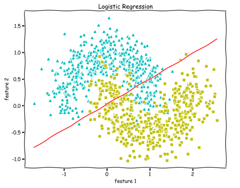
Decision boundary

Now, we want to know how our hypothesis(y_hat) is going to make predictions of whether y=1 or y=0. The way we defined hypothesis is the probability of y being 1 given X and parameterized by w and b .

So, we will say that it will make a prediction of —

y=1 when y_hat ≥ 0.5

y=0 when y_hat < 0.5

Looking at the graph of the sigmoid function, we see that for —

y_hat ≥ 0.5, z or w.X + b ≥ 0

y_hat < 0.5, z or w.X + b < 0

which means, we make a prediction for —

y=1 when w.X + b ≥ 0

y=0 when w.X + b < 0

So, w.X + b = 0 is going to be our Decision boundary.

The following code for plotting the Decision Boundary only works when we have only two features in X.

def plot_decision_boundary(X, w, b):

    # X --> Inputs
    # w --> weights
    # b --> bias

    # The Line is y=mx+c
    # So, Equate mx+c = w.X + b
    # Solving we find m and c
x1 = [min(X[:,0]), max(X[:,0])]
    m = -w[0]/w[1]
    c = -b/w[1]
    x2 = m*x1 + c

    # Plotting
fig = plt.figure(figsize=(10,8))
    plt.plot(X[:, 0][y==0], X[:, 1][y==0], "g^")
    plt.plot(X[:, 0][y==1], X[:, 1][y==1], "bs")
    plt.xlim([-2, 2])
    plt.ylim([0, 2.2])
    plt.xlabel("feature 1")
    plt.ylabel("feature 2")
    plt.title('Decision Boundary')    plt.plot(x1, x2, 'y-')

Normalize Function

Function to normalize the inputs. See comments(#).

def normalize(X):

    # X --> Input.

    # m-> number of training examples
    # n-> number of features 
m, n = X.shape

    # Nrmalizing all the n features of X.
for i in range(n):
        X = (X - X.mean(axis=0))/X.std(axis=0)

   return X

Train Function

The train the function includes initializing the weights and bias and the training loop with mini-batch gradient descent.

See comments(#).

def train(X, y, bs, epochs, lr):

    # X --> Input.
    # y --> true/target value.
    # bs --> Batch Size.
    # epochs --> Number of iterations.
    # lr --> Learning rate.

    # m-> number of training examples
    # n-> number of features 
m, n = X.shape

    # Initializing weights and bias to zeros.
w = np.zeros((n,1))
    b = 0

    # Reshaping y.
y = y.reshape(m,1)

    # Normalizing the inputs.
x = normalize(X)

    # Empty list to store losses.
losses = []

    # Training loop.
 for epoch in range(epochs):
        for i in range((m-1)//bs + 1):

            # Defining batches. SGD.
start_i = i*bs
            end_i = start_i + bs
            xb = X[start_i:end_i]
            yb = y[start_i:end_i]

            # Calculating hypothesis/prediction.
            y_hat = sigmoid(np.dot(xb, w) + b)
            
            # Getting the gradients of loss w.r.t parameters.
            dw, db = gradients(xb, yb, y_hat)
            
            # Updating the parameters.
w -= lr*dw
            b -= lr*db

        # Calculating loss and appending it in the list.
l = loss(y, sigmoid(np.dot(X, w) + b))
        losses.append(l)

    # returning weights, bias and losses(List).
  return w, b, losses

Predict Function

See comments(#).

def predict(X):

    # X --> Input.

    # Normalizing the inputs.
 x = normalize(X)

    # Calculating presictions/y_hat.
    preds = sigmoid(np.dot(X, w) + b)
    
    # Empty List to store predictions.
    pred_class = []    # if y_hat >= 0.5 --> round up to 1
    # if y_hat < 0.5 --> round up to 1
    pred_class = [1 if i > 0.5 else 0 for i in preds]
    
    return np.array(pred_class)

Training and Plotting Decision Boundary

# Training 
w, b, l = train(X, y, bs=100, epochs=1000, lr=0.01)# Plotting Decision Boundary
plot_decision_boundary(X, w, b)

Image by Author

Calculating Accuracy

We check how many examples did we get right and divide it by the total number of examples.

def accuracy(y, y_hat):
    accuracy = np.sum(y == y_hat) / len(y)
    return accuracyaccuracy(X, y_hat=predict(X))
>> 1.0

We get an accuracy of 100%. We can see from the above decision boundary graph that we are able to separate the green and blue classes perfectly.

AI/ML

Trending AI/ML Article Identified & Digested via Granola by Ramsey Elbasheer; a Machine-Driven RSS Bot

via WordPress https://ramseyelbasheer.io/2021/04/08/logistic-regression-from-scratch-in-python/