How do machines plan? —An overview
Original Source Here
How do machines plan? —An overview
A gentle introduction to graph search algorithms and Markov Decision Processes
The ability to plan into the future seems to be one of the key characteristics of intelligence. Physical actions such as walking, cycling, doing sports, or driving requires immense coordination, and the best possible moves depend highly on the external environment (you have to adapt and change your strategy if there is a stone, an obstacle or an opponent in your way). Moreover, most of the things we do day to day — commuting, shopping, cooking, studying, working, etc. — involve both short and long-term planning. Strategic games such as chess and Go are also famous examples where thinking ahead plays a crucial role.
Back in the 1950s, people have come up with mathematical ways to describe the procedure of planning. Now the variants of these methods can be found everywhere, from robot motion planning to finding the best route on Google Maps. In this article, we will look at some of the key formulations and planning algorithms, laying the foundation for future articles on planning and reinforcement learning (RL).
States, actions and rewards (costs)
It is easiest to visualise what a typical planning problem would look like in a navigation setting. Imagine that you are in a maze. You are at some location (x, y) and you can move in four directions — up, down, left and right — as long as you don’t run into a wall. If you reach the target you successfully terminate.
We describe the current situation we are in as states. If you are in location (x, y), x and y can be considered to be encoding the state you are in, because as long as you know x and y, assuming that the maze environment doesn’t change, we will be able to place ourselves at the right location and reconstruct the current situation. Typically, we think of states as a set of details that sufficiently summarises a specific situation we may encounter, and can be used to distinguish one unique situation from another.
If you think of a more realistic robot, you can summarise its configurations using a set of numbers— its pose (location and angle) and all the angles of its many joints, which can be considered states.
Once we are happy with our definition of states, we can think of moving between different states to reach a state we desire. For the example above, this would be reaching the location of the treasure chest. We can move between states by taking actions. In the above case, the actions that the robot can take are limited to moving up, down, left and right. But this doesn’t limit us from thinking of more complicated actions, such as taking longer strides or jumping over hedges, although we won’t consider them for now.
The final ingredient to the problem of planning is the idea of “cost” or “reward”. In shortest path search or in robotics, it is more typical to think of costs of each move, and try to minimise the total cost along the path. In the context of planning in games or environments where you can potentially boost up your scores, energy levels, net worth, etc., it is more common to think of rewards and trying to maximise the total rewards you can collect.
Planning as a search problem
Earlier work in planning have focussed on problems with a finite number of states, with each action leading to a deterministic transition between states. In other words, whenever you take an action, you can be confident of which state you will go to next. This is exactly like the grid maze problem we have just seen.
Because we want to evaluate the shortest path to the target, we assign a cost of 1 to each move and try to minimise the total cost before reaching the target. We can now convert our grid maze problem into a shortest path problem for the state transitions illustrated below on the left. The shortest path that can take us from the initial state to the target state will also minimise the total transition cost.
In a more general case, we can solve shortest path problems for any given connected network (e.g. houses connected by paths on the right). These kind of networks are called “graphs” in maths. There are nodes (in blue) which represents states, and edges (in brown) which represents transitions between states. Graph search algorithms such as Dijkstra and A* can find optimal solutions to shortest path problems on a graph. Dijkstra’s algorithm come with the least amount of assumptions, whereas A* can be more efficient in its search if you have a rough guess (heuristics) of the priorities of expanding the nodes.
In the interest of the length of this article, I will move onto a more general formulation of planning, which is Markov Decision Processes. However, graph search algorithms are very important for solving complex real-world problems such as robotics and shortest path search. If you want to learn more about Dijkstra’s algorithm and A*, I recommend this article with amazing interactive graphics.
How to describe a more general planning problem
Graph search algorithms are great when you have a finite number of states with deterministic transitions between them. However, what if there’s some uncertainty in the transitions, or if there are an infinite number of states and transitions that can be made?
Let’s look at a slightly more involved example of planning — chess. What would states and actions look like in this context?
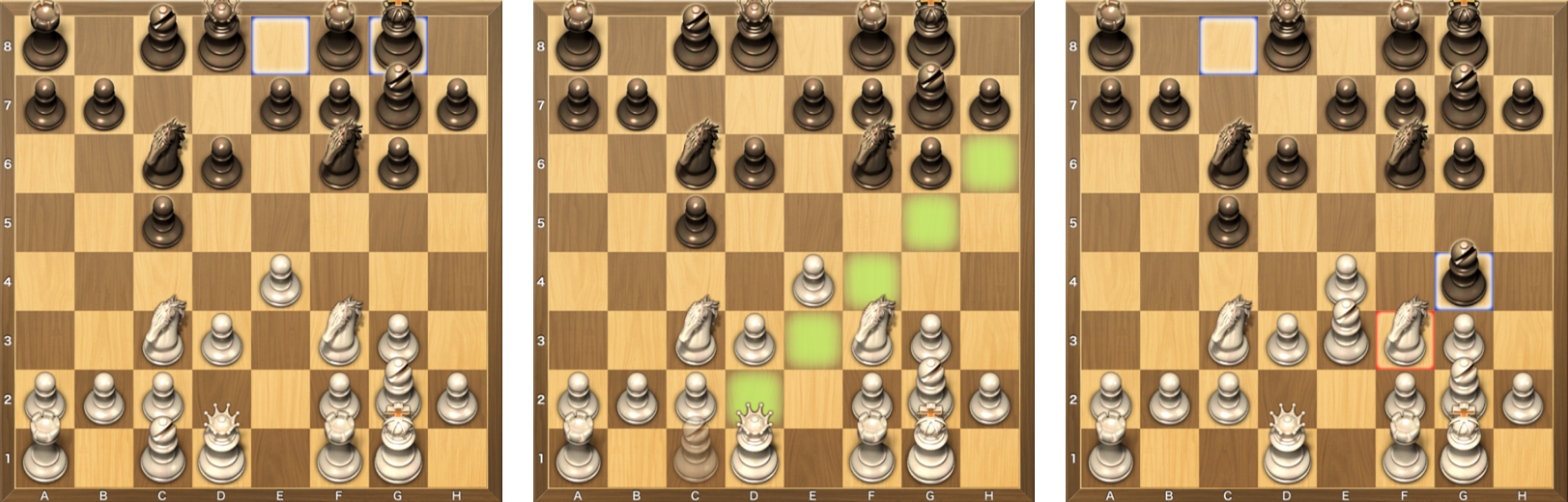
Since each state should capture unique details about the current situation, a plausible choice may be to encode locations of every piece on the board ({‘black king’: G8, ‘black queen’: D8, …, ‘white king’: G1, ‘white queen’: D1…}). The exact way of encoding this is not too important, as long as they have a one-to-one mapping with the board state, and indeed, many chess game engines have come up with different ways of encoding the board state.
There are more possible actions in chess (what you can do to move from one state to another). On average, there are about 30 moves you can make per turn, because you can choose which piece to move and each piece has a set of moves they can make. Let’s say we chose the bishop. The actions we can take in this case are highlighted in green. Once we choose an action, we end up in the next board state, shown on the right.
The interesting thing here is that, because chess is a two-player game, we cannot fully determine the next game state by just choosing our action. The opponent gets to make a move as well, so while we have some idea of what possible next states we can end up in, which state that would be is opened to some uncertainty.
As with most games, there are game states that are more desirable in chess. The most obvious ones are those states when you’ve taken the opponent’s king and you’ve won. The less obvious ones are those where you haven’t won yet but are very close to winning.
Finally, let’s imagine a more real-world problem of driving through some obstacle course. As we’ve discussed, the state of the car can be summarised by its pose (location and angle) as well as the wheel velocity, acceleration, steering angle, the amount of fuel remaining, etc. Actions that take the car from one state to another may be how much you accelerate, break, steer, and top up the fuel.
What makes it difficult in driving or robotics in general is that, unlike the grid maze example or chess, the states and the actions are often continuous. If you are driving the car, you don’t just steer fully to the left or fully to the right; you can accelerate, break, or rotate the steering wheel smoothly, and the resulting position, velocity, acceleration and angle of the car and its wheels all take continuous values. This makes planning in this state space a very hard problem to solve.
Similarly to chess, driving is a multi-agent planning problem, meaning that you have to coordinate with others on the streets who are also driving, cycling or walking. Since we don’t have telepathy yet, we have to make decisions without the full knowledge of what others might decide. There are also environment states that are not fully-known to us, such as when the traffic lights will change next, whether there is a traffic jam in the next intersection, or where exactly we are at right now if we are in a tunnel and don’t have GPS signal.
In the real world, there are many more planning problems that are difficult to solve. What if you are on a road trip and your goal is to visit as many scenic places as possible? There isn’t a single obvious target to be reached in this case. What if you want your AI to learn the best strategy for stock investment, and keep reinvesting your earnings? At which point would you even evaluate the AI’s performance if there isn’t a clear end to this task?
Range of planning problems
We have already seen a lot of similarities and differences in planning problems we might be interested in solving. There are many more assumptions we have made in some of our examples, and adding or removing assumptions can make the problem look entirely different, and with different problems, different solutions arise.
Commonalities:
- The aim is to find a good strategy that allows us to decide which actions to take under a given situation (at a given state)
- There is some kind of mapping between distinct situations and states
- Actions can influence a transition from one state to another
- There is some kind of reward or cost that can be gathered during each transition
- There is a notion of desirability (value) of being in a certain state
Different assumptions depending on the problem:
- Sometimes, it is uncertainty in which state you will end up in after you take an action, either because the state transition is noisy / probabilistic, or because there are others who are also making decisions. There are algorithms developed specifically for two-player games, such as minimax and alpha-beta pruning. In a more general case, we can model a probabilistic state transition as a Markov Decision Process (MDP), which we will discuss next. The problem involving other agents is called a multi-agent problem, and there can be additional considerations that can be made based on whether the agents are cooperating or competing, and whether they are allowed to communicate with each other.
- Sometimes, the rewards you can get for each transition can also be probabilistic.
- In many cases, the state transition and reward dynamics of the environment are unknown until you try things out and see what happens, so it is difficult to plan things ahead without some trial-and-error. This is the main assumption of reinforcement learning, and this dilemma is referred to as “exploitation vs exploration”.
- Sometimes, the states and/or actions can be continuous, which means that discrete planning algorithms such as Dijkstra and A* would no longer work. In robotics, one common approach is to discretise or sample the state space, produce a rough shortest trajectory estimate, and then apply control theory to find a suitable continuous control input that minimises the error between the trajectory estimate and the actual trajectory taken by the robot. With the success of deep learning, however, it has become possible to model a continuous function using neural networks, opening up a range of possibilities to directly plan in continuous space.
- Sometimes, the state we are in cannot be measured exactly. In robotics, where there is limited range of sensor inputs, the most common problem is localisation, i.e. knowing exactly where the robot is at the moment. A Kalman filter is one of the techniques used to estimate the state, given some noisy measurements and observations. SLAM (Simultaneous Localisation and Mapping) is an entire field dedicated to estimating the current position of the robot from camera inputs. More generally, the true state is unknown because we cannot observe the states directly (like whether we have cancer, or the exact position and velocity of every particle in the universe), so we have to estimate them based on a limited amount of observations. A relevant field in reinforcement learning is called POMDP (Partially Observable Markov Decision Process).
These are the motivation for introducing a more general planning paradigm which takes into account these uncertainties — Markov Decision Processes.
Markov Decision Process (MDP)
Let us think of a general planning problem. Whether that be a robot, chess or driving, there is always a decision making entity that changes the situation by taking actions. We call the decision making entity an agent, and everything external to it the environment. Usually, we humans are the agent if we are the ones playing chess, moving around a room or driving. When we solve these problems using an algorithm, the computer algorithms themselves become the agent. The agent can take actions in the environment to reach a new state. The environment is something that provides the agent knowledge about the current state, as well as and the rewards for every state transition that the agent initiates.
States s ∈ S (we denote the set of possible states as S, and each state as s), as described before, is a unique encoding of a specific situation. The current state can either be directly measured or observed (as with chess where the board state is fully known, or a robot arm with fully-known configurations of joints) or has to be inferred from observations provided by the environment (as with driving, where the driver has to infer the current position and velocity of the car, or with a robot which isn’t fully localised).
The agent can initiate transitions from one state to another by taking actions a ∈ A(s) (the actions that are available can depend on which state you are in, so the set of actions can be a function of state s). This will trigger a change in the environment, and the environment will update the agent with observations of the new state, as well as a reward r. The reward can be positive, such as when you made a move resulting in check-mate in chess or correctly predicting the rise in stock, but can also be negative, such as loosing the game, running out of fuel or driving into an obstacle. The rewards are usually a function of the current state s, the action taken by the agent a, and the new state s’, and is written as R(s, a, s’).
Finally, we can also define a transition probability from the current state s to the new state s’, based on some action a as P(s’|s, a). This is a conditional probability because we want to know which state we will end up in, given that we are in state s and have taken the action a.
Let’s illustrate this with a hypothetical scenario where we want to decide whether it is better to going to school by flying on brooms or by teleportation. (Note: I was initially going for a more daily example, but it was difficult to come up with probabilities which are both plausible and easy to inspect, so let’s go with a hypothetical example.)
As illustrated, your starting state s is “home”, and there are three outcomes — school, hospital and kidnapped. If you teleport, it is faster so the rewards for getting to school is higher, but it is riskier so you are more likely to end up in hospital with a severe injury. On the other hand, travelling by broom is slower and is more exposed so there is a chance that you will be kidnapped by aliens.
Let’s decide whether we should take an action “travel by broom” or “teleport”. We can calculate the expectation of rewards (the rewards averaged over the probabilities) for each action (Σ P(s’|s, a)R(s, a, s’))
a=“broom”: 0.8 * 1 + 0.1 * (-10) + 0.1 * (-100) = -10.2
a=“teleport”: 0.7 * 5 + 0.25 * (-15) + 0.05 * (-100) = -5.25
Therefore, in this simple example we found that teleportation gives us the maximum amount of expected rewards for this single move.
Maximising the total expected rewards
While the above example just had a single step of transitions with immediate rewards, in a typical planning problem such as chess, you need to plan ahead and take actions strategically based on your future reward estimates, not just the immediate rewards. More specifically, we should maximise the sum of the rewards we expect in the future. The sum of future rewards are referred to as returns G, and our objective is to find a strategy that maximises it.
Back to our grid maze example, the return at the starting point will be the sum of all the costs to move around and the final reward for reaching the target. Let’s say that the robot took 6 steps to reach the treasure chest, and receives a reward of -1 at every step, but receives a reward of 10 when it reaches the treasure chest. In this case the return is (-1) * 6 + 10 = 4.
Note that in the definition of return, there is a discount factor γ. Some planning problems have no definite end, so rewards keep accumulating indefinitely. To prevent the return to become infinity, we discount future rewards by multiplying γ < 1 (something like γ≈0.99 would do).
Thoughts
I hope this has been helpful to gain some intuition as to how planning problems can be described mathematically, and how the formulation of planning with an MDP is more complex than graph search, but that also allows us to model a more general planning problem.
Usually, the concepts of states, actions and rewards are introduced as a part of the MDP formulation, used in reinforcement learning. In this article, however, I wanted to introduce the idea of states, actions and rewards (costs) more generally, because those ideas are not unique to RL or MDPs, but also appear in robotics, control theory and probability theory, which all have a long history and a lot of great work. Once we start to see these relationships, we start to see that e.g. cumulative costs in Dijkstra’s algorithm and values in reinforcement learning are identical under some assumptions, only formulated in different ways.
In future articles, we will examine reinforcement learning in more depth, look at different methods to arrive at a good strategy, and discuss the intuitions behind them.
References
Related articles
AI/ML
Trending AI/ML Article Identified & Digested via Granola by Ramsey Elbasheer; a Machine-Driven RSS Bot
via WordPress https://ramseyelbasheer.io/2021/04/16/how-do-machines-plan-an-overview/


