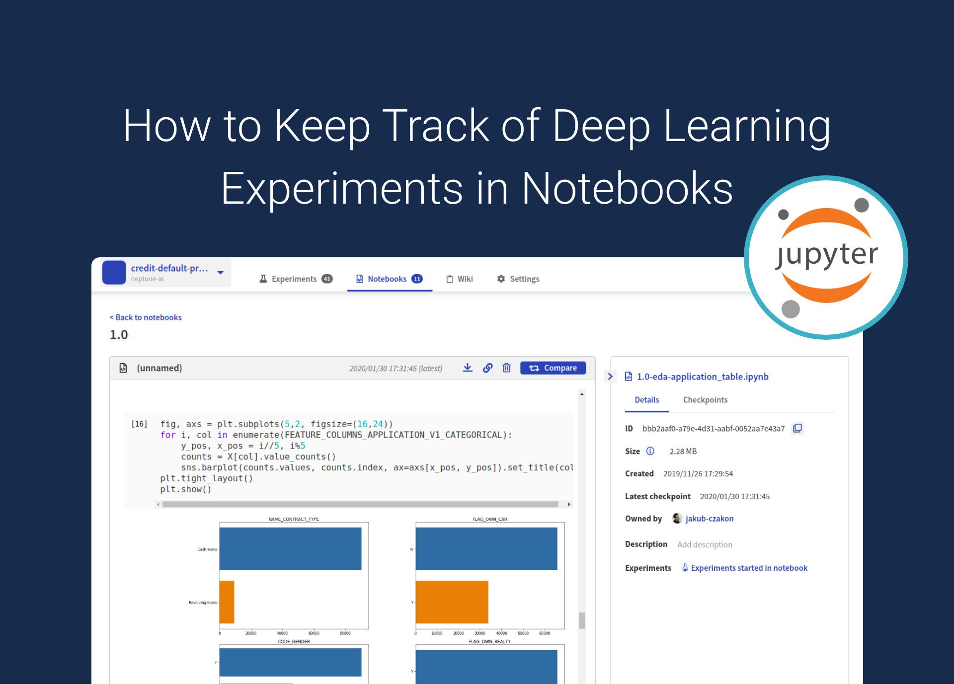
How to Keep Track of Deep Learning Experiments in Notebooks

Original Source Here

Trials are simply training iterations on a specific variable set.

Trial components include various parameters, jobs, datasets, models, metadata, and other artifacts. These can be associated with trials, or they can be independent.

Furthermore, ML flow tracking is an essential part of the experiments we conduct. It is recommended we understand how to use ML flow tracking before continuing on to the tutorial.

There are two components of ML flow tracking: experiments and runs.

An experiment is the primary unit of organization and access control for ML flow runs. All ML flow runs belong to an experiment. Experiments let you visualize, search for, and compare runs, as well as download run artifacts and metadata for analysis in other tools.

Runs, on the other hand, correspond to a single execution of model code. Each run records the source, version, start and end time, parameters, metrics, tags, and artifacts. The source is the name of the notebook that launched the run, or the project name and entry point for the run.

That’s not all. Other important terms include:

• Version: Notebook revision if run from a notebook or Git commit hash if run from an ML Project.
• Start & end time: Start and end time of a run.
• Parameters: Model parameters saved as key-value pairs. Both keys and values are strings.
• Metrics: Model evaluation metrics saved as key-value pairs. The value is numeric. Each metric can be updated throughout the course of the run (for example, to track how your model’s loss function is converging), and ML flow records and lets you visualize the metric’s history.
• Tags: Run metadata saved as key-value pairs. You can update tags during and after a run completes. Both keys and values are strings.
• Artifacts: Output files in any format. For example, you can record images, models (like a pickled scikit-learn model), and data files (like a Parquet file) as an artifact.

Tutorial: tracking Deep Learning experiments in Jupyter Notebooks with Neptune

First, let’s create an experiment in Neptune. Neptune helps you with experiment management, or basically tracking experiment metadata (such as code versions, data versions, hyperparameters, environments, and metrics).

neptune.create_experiment(
    name = 'experiment-example',
    params={'learning_rate':0.1}
)

Logging as many metrics as you can will save your future self a lot of trouble when metrics change with new discoveries or specifications.

Different evaluation metrics include classification accuracy, logarithmic loss, confusion matrix, area under curve, F1 Score, mean absolute error, mean squared error. Tracking these can help you evaluate the performance of your machine learning algorithm and model.

For example, your DL model may give you an appropriate accuracy score, but a poor logarithmic loss. Neptune keeps all these metrics nicely organized for each experiment.

You can log a simple metric such as accuracy with Neptune:

neptune.log_metric('classification_accuracy', 0.99)

You can also log more complex metrics such as a confusion matrix:

neptune.log_metric('diagnostics', 'confusion_matrix.png')

Now, let’s go through a deep learning example where we log metrics after each batch and epoch.

More advanced DL models will go through hundreds of epochs. Manually tracking accuracy, batch loss, and other metrics after each epoch is impossible.

If your model performance is not great, you must figure out if you need more data, reduce the model complexity, or find another solution.

To determine the next step, you must know if your model has a bias or variance problem. If it does, we can use data preprocessing techniques to troubleshoot it.

Learning curves show the relationship between training set size and a chosen evaluation metric, and can be useful for diagnosing model performance. Neptune automatically generates learning curves as the model trains, and logs metrics after each epoch or batch.

But first, you must create a NeptuneLogger callback:

from tensorflow.keras.callbacks import Callback
class NeptuneLogger(Callback):
def on_batch_end(self, batch, logs={}):
for log_name, log_value in logs.items():
           neptune.log_metric(f'batch_{log_name}', log_value)
def on_epoch_end(self, epoch, logs={}):
for log_name, log_value in logs.items():
           neptune.log_metric(f'epoch_{log_name}', log_value)

Next, create an experiment, give it a name, and log some hyperparameters.

Here, we made the epoch size 7, and the batch size 40.

EPOCH_NR = 7
BATCH_SIZE = 40neptune.create_experiment(name='keras-metrics',
                         params={'epoch_nr': EPOCH_NR,
                                 'batch_size': BATCH_SIZE},
                         tags=['advanced'],
                         )

Finally, pass the Neptune logger as Keras callback:

history = model.fit(x=x_train,
                   y=y_train,
                   epochs=EPOCH_NR,
                   batch_size=BATCH_SIZE,
                   validation_data=(x_test, y_test),
                   callbacks=[NeptuneLogger()])

Inside Neptune, you can monitor your learning curves as they train, which is a unique feature that makes it easy for you to observe efficiency.

What’s next?

Jupyter notebooks are great tools for machine learning, but the best way to work with them is to use a platform like Neptune.

The features and affordability make Neptune the least problematic platform on the market.

If you want to learn more about it, and about experiment management within Neptune, check out these resources:

That’s it from me. Thanks for reading!

AI/ML

Trending AI/ML Article Identified & Digested via Granola by Ramsey Elbasheer; a Machine-Driven RSS Bot

via WordPress https://ramseyelbasheer.wordpress.com/2021/03/05/how-to-keep-track-of-deep-learning-experiments-in-notebooks/