Predicting Price of Electricity using Machine Learning
Original Source Here
Predicting Price of Electricity using Machine Learning
Context
Dataset containing the price of electricity for a data center in addition to factors that might affect the price.
Column Descriptions:
DateTime: String, defines date and time of sample
Holiday: String, gives name of holiday if day is a bank holiday
HolidayFlag: integer, 1 if day is a bank holiday, zero otherwise
DayOfWeek: integer (0–6), 0 monday, day of week
WeekOfYear: integer, running week within year of this date
Day integer: day of the date
Month integer: month of the date
Year integer: year of the date
PeriodOfDay integer: denotes half hour period of day (0–47)
SystemLoadEA: the national load forecast for this period
SMPEA: the price forecast for this period
ORKTemperature: the actual temperature measured at Cork airport
ORKWindspeed: the actual windspeed measured at Cork airport
CO2Intensity: the actual CO2 intensity in (g/kWh) for the electricity produced
ActualWindProduction: the actual wind energy production for this period
SystemLoadEP2: the actual national system load for this period
SMPEP2: the actual price of this time period, the value to be forecasted
Research paper
https://www.sciencedirect.com/science/article/pii/S030626191830196X
Importing the necessary libraries
import numpy as np
import pandas as pd
from sklearn.model_selection import train_test_split
from sklearn.metrics import mean_squared_error
from math import sqrt
import keras
from keras.models import Sequential
from keras.layers import Dense
from sklearn.preprocessing import StandardScaler
Reading the dataset
df = pd.read_csv("/content/electricity_prices.csv", na_values=['?'])
df.head()df.shape
(38014, 18)
The dataset contains 38014 rows and 18 columns.
df.info()<class 'pandas.core.frame.DataFrame'>
RangeIndex: 38014 entries, 0 to 38013
Data columns (total 18 columns):
 #   Column                  Non-Null Count  Dtype
---  ------                  --------------  -----
 0   DateTime                38014 non-null  object
 1   Holiday                 38014 non-null  object
 2   HolidayFlag             38014 non-null  int64
 3   DayOfWeek               38014 non-null  int64
 4   WeekOfYear              38014 non-null  int64
 5   Day                     38014 non-null  int64
 6   Month                   38014 non-null  int64
 7   Year                    38014 non-null  int64
 8   PeriodOfDay             38014 non-null  int64
 9   ForecastWindProduction  38009 non-null  float64
 10  SystemLoadEA            38012 non-null  float64
 11  SMPEA                   38012 non-null  float64
 12  ORKTemperature          37719 non-null  float64
 13  ORKWindspeed            37715 non-null  float64
 14  CO2Intensity            38007 non-null  float64
 15  ActualWindProduction    38009 non-null  float64
 16  SystemLoadEP2           38012 non-null  float64
 17  SMPEP2                  38012 non-null  float64
dtypes: float64(9), int64(7), object(2)
memory usage: 5.2+ MB
Checking the Null values
df.isnull().sum()DateTime                    0
Holiday                     0
HolidayFlag                 0
DayOfWeek                   0
WeekOfYear                  0
Day                         0
Month                       0
Year                        0
PeriodOfDay                 0
ForecastWindProduction      5
SystemLoadEA                2
SMPEA                       2
ORKTemperature            295
ORKWindspeed              299
CO2Intensity                7
ActualWindProduction        5
SystemLoadEP2               2
SMPEP2                      2
dtype: int64
ForecastWindProduction , SystemLoadEA , SMPEA ,ORKTemperature ,ORKWindspeed ,CO2Intensity ActualWindProduction , SystemLoadEP2 and SMPEP2 have null values.
Removing the null values
df = df.dropna()
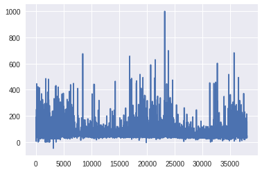
Plotting the target feature
plt.plot("SMPEP2", data=df)
Correlation plot of Independent attributes
plt.figure(figsize=(9,7))
sns.heatmap(df.corr(), annot=True, square=True, fmt='.1f', cbar=False);
Distribution plot of Target feature
sns.distplot(df['SMPEP2'])
Splitting the independent features and target feature
X = df[['ActualWindProduction', 'SystemLoadEP2', 'SMPEA', 'SystemLoadEA', 'ForecastWindProduction',
     'DayOfWeek', 'Year', 'ORKWindspeed', 'CO2Intensity', 'PeriodOfDay']]y = df['SMPEP2']
Train-Validation Split (90% Train set and 10% Validation set)
X_train, X_test, y_train, y_test = train_test_split(X, y, test_size = 0.1, random_state = 42)
sc = StandardScaler()
X_train = sc.fit_transform(X_train)
X_test = sc.transform(X_test)
Model Building using Neural networks
model = keras.Sequential([
        keras.layers.Dense(512, activation="relu", input_shape=[10]),
        keras.layers.Dense(800, activation="relu"),
        keras.layers.Dropout(0.3),
        keras.layers.Dense(1024, activation="relu"),
        keras.layers.Dropout(0.3),
        keras.layers.Dense(1, activation = 'linear'),
        ])
model.summary()Model: "sequential_1"
_________________________________________________________________
Layer (type)                 Output Shape              Param #
=================================================================
dense_4 (Dense)              (None, 512)               5632
_________________________________________________________________
dense_5 (Dense)              (None, 800)               410400
_________________________________________________________________
dropout_2 (Dropout)          (None, 800)               0
_________________________________________________________________
dense_6 (Dense)              (None, 1024)              820224
_________________________________________________________________
dropout_3 (Dropout)          (None, 1024)              0
_________________________________________________________________
dense_7 (Dense)              (None, 1)                 1025
=================================================================
Total params: 1,237,281
Trainable params: 1,237,281
Non-trainable params: 0
Compiling the model
model.compile(loss='mse', optimizer='adam', metrics=['mse','mae'])
Fitting the model with Early stopping and restoring the best weights
early_stopping = keras.callbacks.EarlyStopping(patience = 10, min_delta = 0.001, restore_best_weights =True )history = model.fit(
    X_train, y_train,
    validation_data=(X_test, y_test),
    batch_size=50,
    epochs=100,
    callbacks=[early_stopping],
    verbose=1,
)
Evaluating the model on test set
from sklearn.metrics import mean_absolute_error,r2_score
predictions = model.predict(X_test)
print(f"MAE: {mean_absolute_error(y_test, predictions)}")

print(f"R2_score: {r2_score(y_test, predictions)}")
MAE: 10.99616479512835
R2_score: 0.5678318389935775
XG Boost Regressor Model
from xgboost import XGBRegressor
model2 = XGBRegressor(n_estimators = 8000, max_depth=17, eta=0.1, subsample=0.7, colsample_bytree=0.8)
model2.fit(X_train, y_train)
pred = model2.predict(X_test)
r2_score(y_test, pred)
R2 Score is 0.6137340486115418
mean_absolute_error(y_test, pred)
Mean Absolute error is 9.415647364373736
Final Predictions of XG Boost Model
predarray([ 45.052734,  58.09632 ,  66.80695 , ...,  63.155807,  40.944473,
       182.29193 ], dtype=float32)
Dump model to pickle file
model2.predict(X_test)
pkl_out = open("train_classifier","wb")
pkl.dump(model2,pkl_out)
Conclusion
By using this analysis we can predict electricity prices that is the actual price of this time period and forecast future business strategies.
AI/ML
Trending AI/ML Article Identified & Digested via Granola by Ramsey Elbasheer; a Machine-Driven RSS Bot
via WordPress https://ramseyelbasheer.io/2021/06/11/predicting-price-of-electricity-using-machine-learning/


